Performs multivariate multiple regression with mixture-of-normals prior.
mr.mash(
  X,
  Y,
  S0,
  w0 = rep(1/(length(S0)), length(S0)),
  V = NULL,
  mu1_init = matrix(0, nrow = ncol(X), ncol = ncol(Y)),
  tol = 0.0001,
  convergence_criterion = c("mu1", "ELBO"),
  max_iter = 5000,
  update_w0 = TRUE,
  update_w0_method = "EM",
  w0_threshold = 0,
  compute_ELBO = TRUE,
  standardize = TRUE,
  verbose = TRUE,
  update_V = FALSE,
  update_V_method = c("full", "diagonal"),
  version = c("Rcpp", "R"),
  e = 1e-08,
  ca_update_order = c("consecutive", "decreasing_logBF", "increasing_logBF", "random"),
  nthreads = as.integer(NA)
)
Arguments
- X
n x p matrix of covariates.
- Y
n x r matrix of responses.
- S0
List of length K containing the desired r x r prior covariance matrices on the regression coefficients.
- w0
K-vector with prior mixture weights, each associated with the respective covariance matrix in
S0.- V
r x r residual covariance matrix.
- mu1_init
p x r matrix of initial estimates of the posterior mean regression coefficients. These should be on the same scale as the X provided. If
standardize=TRUE, mu1_init will be scaled appropriately after standardizing X.- tol
Convergence tolerance.
- convergence_criterion
Criterion to use for convergence check.
- max_iter
Maximum number of iterations for the optimization algorithm.
- update_w0
If
TRUE, prior weights are updated.- update_w0_method
Method to update prior weights. Only EM is currently supported.
- w0_threshold
Drop mixture components with weight less than this value. Components are dropped at each iteration after 15 initial iterations. This is done to prevent from dropping some poetentially important components prematurely.
- compute_ELBO
If
TRUE, ELBO is computed.- standardize
If
TRUE, X is "standardized" using the sample means and sample standard deviations. Standardizing X allows a faster implementation, but the prior has a different interpretation. Coefficients and covariances are returned on the original scale.- verbose
If
TRUE, some information about the algorithm's process is printed at each iteration.- update_V
if
TRUE, residual covariance is updated.- update_V_method
Method to update residual covariance. So far, "full" and "diagonal" are supported. If
update_V=TRUEand V is not provided by the user, this option will determine how V is computed (and fixed) internally frommu1_init.- version
Whether to use R or C++ code to perform the coordinate ascent updates.
- e
A small number to add to the diagonal elements of the prior matrices to improve numerical stability of the updates.
- ca_update_order
The order with which coordinates are updated. So far, "consecutive", "decreasing_logBF", "increasing_logBF", "random" are supported.
- nthreads
Number of RcppParallel threads to use for the updates. When
nthreadsisNA, the default number of threads is used; seedefaultNumThreads. This setting is ignored whenversion = "R".
Value
A mr.mash fit, stored as a list with some or all of the following elements:
- mu1
p x r matrix of posterior means for the regression coeffcients.
- S1
r x r x p array of posterior covariances for the regression coeffcients.
- w1
p x K matrix of posterior assignment probabilities to the mixture components.
- V
r x r residual covariance matrix
- w0
K-vector with (updated, if
update_w0=TRUE) prior mixture weights, each associated with the respective covariance matrix inS0
.
- S0
r x r x K array of prior covariance matrices on the regression coefficients
.
- intercept
r-vector containing posterior mean estimate of the intercept.
- fitted
n x r matrix of fitted values.
- G
r x r covariance matrix of fitted values.
- pve
r-vector of proportion of variance explained by the covariates.
- ELBO
Evidence Lower Bound (ELBO) at last iteration.
- progress
A data frame including information regarding convergence criteria at each iteration.
- converged
TRUEorFALSE, indicating whether the optimization algorithm converged to a solution within the chosen tolerance level.- Y
n x r matrix of responses at last iteration (only relevant when missing values are present in the input Y).
Examples
###Set seed
set.seed(123)
###Simulate X and Y
##Set parameters
n <- 1000
p <- 100
p_causal <- 20
r <- 5
###Simulate data
out <- simulate_mr_mash_data(n, p, p_causal, r, pve=0.5, B_cor=1,
B_scale=1, X_cor=0, X_scale=1, V_cor=0)
###Split the data in training and test sets
Ytrain <- out$Y[-c(1:200), ]
Xtrain <- out$X[-c(1:200), ]
Ytest <- out$Y[c(1:200), ]
Xtest <- out$X[c(1:200), ]
###Specify the covariance matrices for the mixture-of-normals prior.
univ_sumstats <- compute_univariate_sumstats(Xtrain, Ytrain,
standardize=TRUE, standardize.response=FALSE)
grid <- autoselect.mixsd(univ_sumstats, mult=sqrt(2))^2
S0 <- compute_canonical_covs(ncol(Ytrain), singletons=TRUE,
hetgrid=c(0, 0.25, 0.5, 0.75, 1))
S0 <- expand_covs(S0, grid, zeromat=TRUE)
###Fit mr.mash
fit <- mr.mash(Xtrain, Ytrain, S0, update_V=TRUE)
#> Processing the inputs... Done!
#> Fitting the optimization algorithm using 8 RcppParallel threads...
#> iter mu1_max.diff ELBO_diff ELBO
#> 1 1.94e+00 Inf -1.17846672180838359054e+04
#> 2 4.42e-01 4.05e+02 -1.13796024149418335583e+04
#> 3 7.87e-02 2.57e+01 -1.13539336653549289622e+04
#> 4 2.58e-02 2.82e+00 -1.13511145933636835252e+04
#> 5 1.32e-02 1.31e+00 -1.13498072316737907386e+04
#> 6 8.97e-03 7.79e-01 -1.13490277534703436686e+04
#> 7 7.04e-03 5.18e-01 -1.13485098880874957104e+04
#> 8 5.70e-03 3.70e-01 -1.13481397449429277913e+04
#> 9 4.72e-03 2.79e-01 -1.13478605353105485847e+04
#> 10 3.99e-03 2.19e-01 -1.13476411012395928992e+04
#> 11 3.42e-03 1.78e-01 -1.13474630689185141819e+04
#> 12 2.97e-03 1.48e-01 -1.13473149520036367903e+04
#> 13 2.61e-03 1.26e-01 -1.13471892144920439023e+04
#> 14 2.32e-03 1.09e-01 -1.13470807090191228781e+04
#> 15 2.07e-03 9.49e-02 -1.13469857987776576920e+04
#> 16 1.87e-03 8.40e-02 -1.13469018391313620668e+04
#> 17 1.69e-03 7.50e-02 -1.13468268583168064652e+04
#> 18 1.57e-03 6.75e-02 -1.13467593534742900374e+04
#> 19 1.48e-03 6.12e-02 -1.13466981562588171073e+04
#> 20 1.40e-03 5.58e-02 -1.13466423419556540466e+04
#> 21 1.36e-03 5.12e-02 -1.13465911666470801720e+04
#> 22 1.36e-03 4.71e-02 -1.13465440229446667217e+04
#> 23 1.35e-03 4.36e-02 -1.13465004082810373802e+04
#> 24 1.32e-03 4.05e-02 -1.13464599018548724416e+04
#> 25 1.30e-03 3.78e-02 -1.13464221476301063376e+04
#> 26 1.26e-03 3.53e-02 -1.13463868416268542205e+04
#> 27 1.22e-03 3.31e-02 -1.13463537222899558401e+04
#> 28 1.18e-03 3.12e-02 -1.13463225630880588142e+04
#> 29 1.14e-03 2.94e-02 -1.13462931667455850402e+04
#> 30 1.09e-03 2.78e-02 -1.13462653606825715542e+04
#> 31 1.05e-03 2.64e-02 -1.13462389933572903828e+04
#> 32 1.00e-03 2.51e-02 -1.13462139312915114715e+04
#> 33 9.57e-04 2.39e-02 -1.13461900566182957846e+04
#> 34 9.13e-04 2.28e-02 -1.13461672650350483309e+04
#> 35 8.69e-04 2.18e-02 -1.13461454640754946013e+04
#> 36 8.27e-04 2.09e-02 -1.13461245716363282554e+04
#> 37 7.87e-04 2.01e-02 -1.13461045147101667681e+04
#> 38 7.48e-04 1.93e-02 -1.13460852282884388842e+04
#> 39 7.10e-04 1.86e-02 -1.13460666544058058207e+04
#> 40 6.75e-04 1.79e-02 -1.13460487413043974811e+04
#> 41 6.41e-04 1.73e-02 -1.13460314427002595039e+04
#> 42 6.09e-04 1.67e-02 -1.13460147171381850058e+04
#> 43 5.78e-04 1.62e-02 -1.13459985274232658412e+04
#> 44 5.50e-04 1.57e-02 -1.13459828401197173662e+04
#> 45 5.23e-04 1.52e-02 -1.13459676251087985293e+04
#> 46 4.97e-04 1.48e-02 -1.13459528551988605614e+04
#> 47 4.73e-04 1.43e-02 -1.13459385057816034532e+04
#> 48 4.51e-04 1.40e-02 -1.13459245545291032613e+04
#> 49 4.30e-04 1.36e-02 -1.13459109811270991486e+04
#> 50 4.11e-04 1.32e-02 -1.13458977670403019147e+04
#> 51 3.98e-04 1.29e-02 -1.13458848953061169595e+04
#> 52 3.85e-04 1.25e-02 -1.13458723503535020427e+04
#> 53 3.72e-04 1.22e-02 -1.13458601178440185322e+04
#> 54 3.61e-04 1.19e-02 -1.13458481845324549795e+04
#> 55 3.49e-04 1.16e-02 -1.13458365381447929394e+04
#> 56 3.38e-04 1.14e-02 -1.13458251672713195148e+04
#> 57 3.28e-04 1.11e-02 -1.13458140612731313013e+04
#> 58 3.18e-04 1.09e-02 -1.13458032102003544423e+04
#> 59 3.08e-04 1.06e-02 -1.13457926047206601652e+04
#> 60 2.99e-04 1.04e-02 -1.13457822360567515716e+04
#> 61 2.90e-04 1.01e-02 -1.13457720959317412053e+04
#> 62 2.82e-04 9.92e-03 -1.13457621765213207254e+04
#> 63 2.73e-04 9.71e-03 -1.13457524704120151000e+04
#> 64 2.66e-04 9.50e-03 -1.13457429705644990463e+04
#> 65 2.58e-04 9.30e-03 -1.13457336702815864555e+04
#> 66 2.51e-04 9.11e-03 -1.13457245631800287811e+04
#> 67 2.44e-04 8.92e-03 -1.13457156431657749636e+04
#> 68 2.37e-04 8.74e-03 -1.13457069044121872139e+04
#> 69 2.30e-04 8.56e-03 -1.13456983413408052002e+04
#> 70 2.24e-04 8.39e-03 -1.13456899486043275829e+04
#> 71 2.17e-04 8.23e-03 -1.13456817210715034889e+04
#> 72 2.11e-04 8.07e-03 -1.13456736538136992749e+04
#> 73 2.06e-04 7.91e-03 -1.13456657420928877400e+04
#> 74 2.00e-04 7.76e-03 -1.13456579813508433290e+04
#> 75 1.95e-04 7.61e-03 -1.13456503671994796605e+04
#> 76 1.89e-04 7.47e-03 -1.13456428954120528942e+04
#> 77 1.84e-04 7.33e-03 -1.13456355619151800056e+04
#> 78 1.79e-04 7.20e-03 -1.13456283627815500950e+04
#> 79 1.74e-04 7.07e-03 -1.13456212942232650676e+04
#> 80 1.70e-04 6.94e-03 -1.13456143525856532506e+04
#> 81 1.66e-04 6.82e-03 -1.13456075343415668613e+04
#> 82 1.63e-04 6.70e-03 -1.13456008360861123947e+04
#> 83 1.60e-04 6.58e-03 -1.13455942545316338510e+04
#> 84 1.56e-04 6.47e-03 -1.13455877865031015972e+04
#> 85 1.57e-04 6.36e-03 -1.13455814289337140508e+04
#> 86 1.59e-04 6.25e-03 -1.13455751788607631170e+04
#> 87 1.60e-04 6.15e-03 -1.13455690334217033524e+04
#> 88 1.61e-04 6.04e-03 -1.13455629898503993900e+04
#> 89 1.62e-04 5.94e-03 -1.13455570454735989188e+04
#> 90 1.62e-04 5.85e-03 -1.13455511977075166214e+04
#> 91 1.63e-04 5.75e-03 -1.13455454440545527177e+04
#> 92 1.64e-04 5.66e-03 -1.13455397821002097771e+04
#> 93 1.64e-04 5.57e-03 -1.13455342095100804727e+04
#> 94 1.65e-04 5.49e-03 -1.13455287240269317408e+04
#> 95 1.65e-04 5.40e-03 -1.13455233234679890302e+04
#> 96 1.65e-04 5.32e-03 -1.13455180057222332834e+04
#> 97 1.65e-04 5.24e-03 -1.13455127687478270673e+04
#> 98 1.66e-04 5.16e-03 -1.13455076105696498416e+04
#> 99 1.66e-04 5.08e-03 -1.13455025292769078078e+04
#> 100 1.66e-04 5.01e-03 -1.13454975230208328867e+04
#> 101 1.66e-04 4.93e-03 -1.13454925900124599139e+04
#> 102 1.66e-04 4.86e-03 -1.13454877285204838699e+04
#> 103 1.66e-04 4.79e-03 -1.13454829368692244316e+04
#> 104 1.66e-04 4.72e-03 -1.13454782134365996171e+04
#> 105 1.66e-04 4.66e-03 -1.13454735566522485897e+04
#> 106 1.65e-04 4.59e-03 -1.13454689649956708308e+04
#> 107 1.65e-04 4.53e-03 -1.13454644369944471691e+04
#> 108 1.65e-04 4.47e-03 -1.13454599712225481198e+04
#> 109 1.64e-04 4.40e-03 -1.13454555662986731477e+04
#> 110 1.64e-04 4.35e-03 -1.13454512208846699650e+04
#> 111 1.64e-04 4.29e-03 -1.13454469336840083997e+04
#> 112 1.63e-04 4.23e-03 -1.13454427034403252037e+04
#> 113 1.62e-04 4.17e-03 -1.13454385289359997842e+04
#> 114 1.62e-04 4.12e-03 -1.13454344089908081514e+04
#> 115 1.61e-04 4.07e-03 -1.13454303424606005137e+04
#> 116 1.61e-04 4.01e-03 -1.13454263282360734593e+04
#> 117 1.60e-04 3.96e-03 -1.13454223652415312245e+04
#> 118 1.59e-04 3.91e-03 -1.13454184524337561015e+04
#> 119 1.58e-04 3.86e-03 -1.13454145888008642942e+04
#> 120 1.58e-04 3.82e-03 -1.13454107733612545417e+04
#> 121 1.57e-04 3.77e-03 -1.13454070051625585620e+04
#> 122 1.56e-04 3.72e-03 -1.13454032832806569786e+04
#> 123 1.55e-04 3.68e-03 -1.13453996068187316268e+04
#> 124 1.54e-04 3.63e-03 -1.13453959749063160416e+04
#> 125 1.53e-04 3.59e-03 -1.13453923866984387132e+04
#> 126 1.52e-04 3.55e-03 -1.13453888413747736195e+04
#> 127 1.52e-04 3.50e-03 -1.13453853381387798436e+04
#> 128 1.51e-04 3.46e-03 -1.13453818762169721595e+04
#> 129 1.50e-04 3.42e-03 -1.13453784548581006675e+04
#> 130 1.49e-04 3.38e-03 -1.13453750733324523026e+04
#> 131 1.48e-04 3.34e-03 -1.13453717309311268764e+04
#> 132 1.47e-04 3.30e-03 -1.13453684269653767842e+04
#> 133 1.46e-04 3.27e-03 -1.13453651607659248839e+04
#> 134 1.45e-04 3.23e-03 -1.13453619316823187546e+04
#> 135 1.44e-04 3.19e-03 -1.13453587390823558962e+04
#> 136 1.42e-04 3.16e-03 -1.13453555823514725489e+04
#> 137 1.41e-04 3.12e-03 -1.13453524608921470644e+04
#> 138 1.40e-04 3.09e-03 -1.13453493741233905894e+04
#> 139 1.39e-04 3.05e-03 -1.13453463214801831782e+04
#> 140 1.38e-04 3.02e-03 -1.13453433024129535625e+04
#> 141 1.37e-04 2.99e-03 -1.13453403163871043944e+04
#> 142 1.36e-04 2.95e-03 -1.13453373628825011110e+04
#> 143 1.35e-04 2.92e-03 -1.13453344413930117298e+04
#> 144 1.34e-04 2.89e-03 -1.13453315514260684722e+04
#> 145 1.33e-04 2.86e-03 -1.13453286925021966454e+04
#> 146 1.32e-04 2.83e-03 -1.13453258641546271974e+04
#> 147 1.31e-04 2.80e-03 -1.13453230659288401512e+04
#> 148 1.30e-04 2.77e-03 -1.13453202973822026252e+04
#> 149 1.29e-04 2.74e-03 -1.13453175580835577421e+04
#> 150 1.27e-04 2.71e-03 -1.13453148476128681068e+04
#> 151 1.26e-04 2.68e-03 -1.13453121655608229048e+04
#> 152 1.25e-04 2.65e-03 -1.13453095115285104839e+04
#> 153 1.24e-04 2.63e-03 -1.13453068851270636515e+04
#> 154 1.23e-04 2.60e-03 -1.13453042859773267992e+04
#> 155 1.22e-04 2.57e-03 -1.13453017137095375801e+04
#> 156 1.21e-04 2.55e-03 -1.13452991679629994906e+04
#> 157 1.20e-04 2.52e-03 -1.13452966483858072024e+04
#> 158 1.19e-04 2.49e-03 -1.13452941546345209645e+04
#> 159 1.18e-04 2.47e-03 -1.13452916863738901156e+04
#> 160 1.17e-04 2.44e-03 -1.13452892432765893318e+04
#> 161 1.16e-04 2.42e-03 -1.13452868250229294063e+04
#> 162 1.15e-04 2.39e-03 -1.13452844313006080483e+04
#> 163 1.14e-04 2.37e-03 -1.13452820618044588628e+04
#> 164 1.13e-04 2.35e-03 -1.13452797162361857772e+04
#> 165 1.12e-04 2.32e-03 -1.13452773943041611346e+04
#> 166 1.11e-04 2.30e-03 -1.13452750957231546636e+04
#> 167 1.10e-04 2.28e-03 -1.13452728202141315705e+04
#> 168 1.09e-04 2.25e-03 -1.13452705675040451752e+04
#> 169 1.08e-04 2.23e-03 -1.13452683373256022605e+04
#> 170 1.07e-04 2.21e-03 -1.13452661294170684414e+04
#> 171 1.06e-04 2.19e-03 -1.13452639435220935411e+04
#> 172 1.05e-04 2.16e-03 -1.13452617793894787610e+04
#> 173 1.04e-04 2.14e-03 -1.13452596367730275233e+04
#> 174 1.03e-04 2.12e-03 -1.13452575154313508392e+04
#> 175 1.03e-04 2.10e-03 -1.13452554151276999619e+04
#> 176 1.02e-04 2.08e-03 -1.13452533356297935825e+04
#> 177 1.01e-04 2.06e-03 -1.13452512767096577591e+04
#> 178 9.98e-05 2.04e-03 -1.13452492381434822164e+04
#> Done!
#> Processing the outputs... Done!
#> mr.mash successfully executed in 0.1873724 minutes!
# Compare the "fitted" values of Y against the true Y in the training set.
plot(fit$fitted,Ytrain,pch = 20,col = "darkblue",xlab = "true",
ylab = "fitted")
abline(a = 0,b = 1,col = "magenta",lty = "dotted")
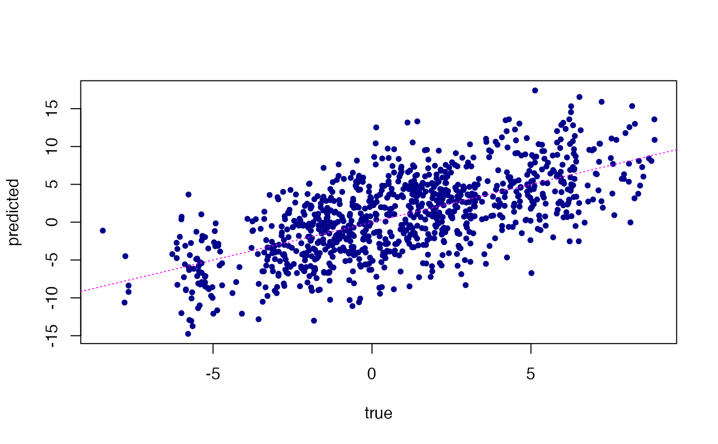
 # Predict the multivariate outcomes in the test set using the fitted model.
Ytest_est <- predict(fit,Xtest)
plot(Ytest_est,Ytest,pch = 20,col = "darkblue",xlab = "true",
ylab = "predicted")
abline(a = 0,b = 1,col = "magenta",lty = "dotted")
# Predict the multivariate outcomes in the test set using the fitted model.
Ytest_est <- predict(fit,Xtest)
plot(Ytest_est,Ytest,pch = 20,col = "darkblue",xlab = "true",
ylab = "predicted")
abline(a = 0,b = 1,col = "magenta",lty = "dotted")