Here we go through a simple example of using Multiple Regression Adaptive Shrinkage, < maybe insert paper link here? >
library(mr.ash)
Step 1: Data Simulation
We simulate a regression data matrix X with n = 400 samples and p = 2000 variables, and a normal response vector y:
set.seed(1)
n <- 400
p <- 1000
pve <- 0.5
s <- 10

## I feel like I shouldn't need to sources these two files, but it keeps saying function
## not found when I knit/build after loading even tho I can use it freely in commandline
source("../R/misc2.R")
source("../R/datasim.R")
sim_data <- simulate_data(n, p, pve, s)
Step 2: Fitting Mr.ASH
This is the most basic usage, using the default settings:
fit <- mr_ash(sim_data$X,sim_data$y,
              control = list(max.iter = 500,convtol = 1e-12),
              verbose = "detailed")

# iter                elbo ||b-b'||   sigma2 w>0
#    1 +2.405642681821e+03 2.96e+00 7.05e-01  20
#    2 +1.327075779103e+03 3.36e-01 5.71e-01  20
#    3 +9.868513871648e+02 2.00e-01 5.93e-01  20
#    4 +8.541453355042e+02 1.37e-01 6.34e-01  20
#    5 +7.866237345676e+02 1.09e-01 6.73e-01  20
#    6 +7.471872913125e+02 8.65e-02 7.04e-01  17
#    7 +7.228338002780e+02 6.18e-02 7.31e-01  13
#    8 +7.069318149041e+02 4.17e-02 7.53e-01  11
#    9 +6.957980471234e+02 2.99e-02 7.72e-01  10
#   10 +6.876027709319e+02 2.20e-02 7.88e-01   9
#  ........
#  490 +6.456370631675e+02 1.15e-07 9.82e-01   3
#  491 +6.456370592689e+02 1.13e-07 9.82e-01   3
#  492 +6.456370554377e+02 1.11e-07 9.82e-01   3
#  493 +6.456370516727e+02 1.09e-07 9.82e-01   3
#  494 +6.456370479728e+02 1.08e-07 9.82e-01   3
#  495 +6.456370443367e+02 1.06e-07 9.82e-01   3
#  496 +6.456370407633e+02 1.04e-07 9.82e-01   3
#  497 +6.456370372514e+02 1.03e-07 9.82e-01   3
#  498 +6.456370338000e+02 1.01e-07 9.82e-01   3
#  499 +6.456370304080e+02 9.95e-08 9.82e-01   3
#  500 +6.456370270742e+02 9.80e-08 9.82e-01   3
# Mr.ASH terminated at iteration 500.
The default model is a mixture with 20 components, with prior mixture component variances in increasing order, starting at zero and ending at roughly 1:
fit$sa2
#>  [1] 0.000000000 0.001249739 0.005176797 0.012064587 0.022220082 0.035975617
#>  [7] 0.053690831 0.075754746 0.102587999 0.134645248 0.172417743 0.216436097
#> [13] 0.267273249 0.325547659 0.391926725 0.467130460 0.551935431 0.647178991
#> [19] 0.753763822 0.872662805
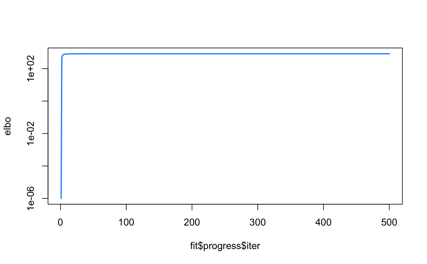
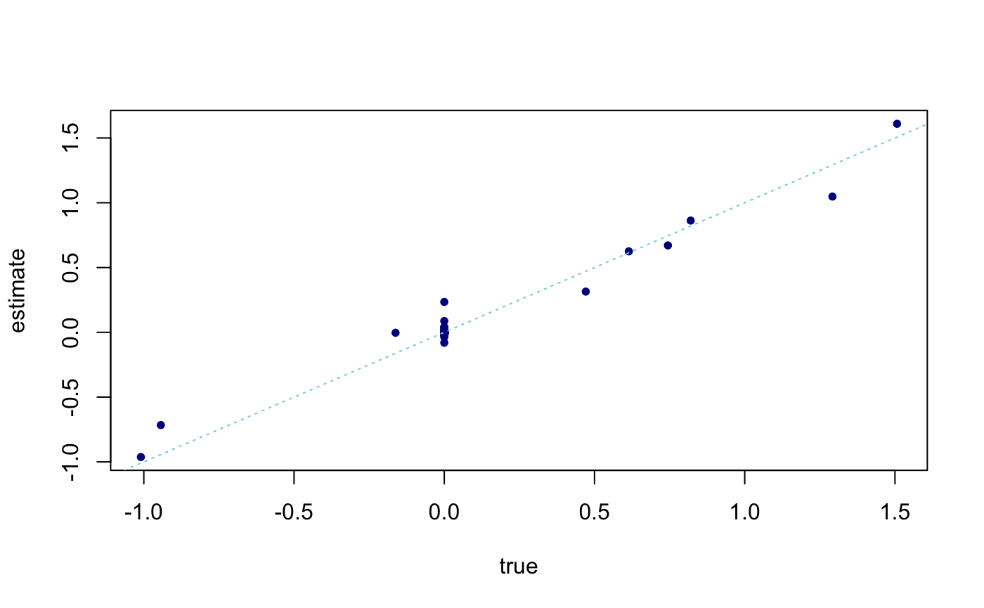
For each iteration, we calculate the Evidence Lower Bound (ELBO) until the maximum iterations specified is reached (in the case demonstrated here), or when convergence criterion is met. We can observe that the estimated \(\beta\) is a good reflection of the
elbo <- fit$progress$elbo
elbo <- elbo - min(elbo) + 1e-6
plot(fit$progress$iter, elbo, type = "l",log = "y",lwd = 2,col = "dodgerblue")
plot(sim_data$beta,coef(fit)[-1],pch = 20,col = "darkblue",xlab = "true",ylab = "estimate")
abline(a = 0,b = 1,col = "skyblue",lty = "dotted")
Step 3: Extract Posterior Summaries
## Another *source* issue
source("../R/misc.R")
posterior <- get_posterior_summary(fit)
str(posterior)
#> List of 3
#>  $ m   : num [1:1000, 1:20] 0 0 0 0 0 0 0 0 0 0 ...
#>  $ s2  : num [1:1000, 1:20] 0 0 0 0 0 0 0 0 0 0 ...
#>  $ lfsr: num [1:1000] 0.998 0.978 0.975 0.996 0.668 ...
#>  - attr(*, "class")= chr [1:2] "posterior" "list"

head(posterior$m)
#>      [,1]        [,2]        [,3]       [,4]       [,5]       [,6]       [,7]
#> [1,]    0 -0.04286624 -0.08865649 -0.1100063 -0.1199269 -0.1250494 -0.1279626
#> [2,]    0 -0.26927406 -0.51759868 -0.6217775 -0.6679596 -0.6912821 -0.7043905
#> [3,]    0 -0.27191562 -0.53657684 -0.6518484 -0.7037841 -0.7302112 -0.7451237
#> [4,]    0  0.11912606  0.23789511  0.2905201  0.3144115  0.3266120  0.3335097
#> [5,]    0  0.41102973  0.79260574  0.9534142  1.0248380  1.0609402  1.0812411
#> [6,]    0  0.26637163  0.52740756  0.6416508  0.6932330  0.7195064  0.7343401
#>            [,8]       [,9]      [,10]      [,11]      [,12]      [,13]
#> [1,] -0.1297504 -0.1309146 -0.1317089 -0.1322716 -0.1326825 -0.1329903
#> [2,] -0.7123805 -0.7175611 -0.7210859 -0.7235777 -0.7253950 -0.7267549
#> [3,] -0.7542343 -0.7601500 -0.7641788 -0.7670288 -0.7691083 -0.7706649
#> [4,]  0.3377283  0.3404695  0.3423371  0.3436588  0.3446233  0.3453454
#> [5,]  1.0936184  1.1016451  1.1071068  1.1109684  1.1137847  1.1158923
#> [6,]  0.7434052  0.7492926  0.7533025  0.7561395  0.7582096  0.7597593
#>           [,14]      [,15]      [,16]      [,17]      [,18]      [,19]
#> [1,] -0.1332259 -0.1334094 -0.1335547 -0.1336713 -0.1337659 -0.1338435
#> [2,] -0.7277947 -0.7286044 -0.7292451 -0.7297589 -0.7301759 -0.7305180
#> [3,] -0.7718555 -0.7727828 -0.7735166 -0.7741052 -0.7745829 -0.7749749
#> [4,]  0.3458978  0.3463281  0.3466686  0.3469418  0.3471635  0.3473454
#> [5,]  1.1175038  1.1187589  1.1197518  1.1205482  1.1211946  1.1217248
#> [6,]  0.7609445  0.7618678  0.7625984  0.7631844  0.7636601  0.7640503
#>           [,20]
#> [1,] -0.1339078
#> [2,] -0.7308013
#> [3,] -0.7752994
#> [4,]  0.3474960
#> [5,]  1.1221639
#> [6,]  0.7643735
head(posterior$s2)
#>      [,1]        [,2]       [,3]       [,4]       [,5]       [,6]       [,7]
#> [1,]    0 0.006170663 0.01276224 0.01583559 0.01726367 0.01800106 0.01842042
#> [2,]    0 0.005731865 0.01101779 0.01323538 0.01421843 0.01471488 0.01499391
#> [3,]    0 0.005892882 0.01162855 0.01412668 0.01525222 0.01582494 0.01614812
#> [4,]    0 0.005964680 0.01191148 0.01454643 0.01574268 0.01635357 0.01669894
#> [5,]    0 0.005751660 0.01109117 0.01334140 0.01434086 0.01484605 0.01513012
#> [6,]    0 0.005913210 0.01170797 0.01424407 0.01538915 0.01597239 0.01630169
#>            [,8]       [,9]      [,10]      [,11]      [,12]      [,13]
#> [1,] 0.01867778 0.01884536 0.01895971 0.01904070 0.01909986 0.01914417
#> [2,] 0.01516399 0.01527427 0.01534929 0.01540234 0.01544102 0.01546997
#> [3,] 0.01634556 0.01647377 0.01656108 0.01662284 0.01666791 0.01670164
#> [4,] 0.01691016 0.01704742 0.01714093 0.01720710 0.01725540 0.01729156
#> [5,] 0.01530332 0.01541564 0.01549207 0.01554611 0.01558552 0.01561501
#> [6,] 0.01650293 0.01663362 0.01672264 0.01678562 0.01683157 0.01686597
#>           [,14]      [,15]      [,16]      [,17]      [,18]      [,19]
#> [1,] 0.01917808 0.01920450 0.01922541 0.01924219 0.01925581 0.01926699
#> [2,] 0.01549210 0.01550934 0.01552297 0.01553391 0.01554279 0.01555007
#> [3,] 0.01672744 0.01674754 0.01676344 0.01677620 0.01678655 0.01679505
#> [4,] 0.01731921 0.01734076 0.01735781 0.01737148 0.01738259 0.01739169
#> [5,] 0.01563756 0.01565512 0.01566902 0.01568016 0.01568921 0.01569663
#> [6,] 0.01689228 0.01691278 0.01692900 0.01694200 0.01695256 0.01696123
#>           [,20]
#> [1,] 0.01927625
#> [2,] 0.01555610
#> [3,] 0.01680208
#> [4,] 0.01739924
#> [5,] 0.01570277
#> [6,] 0.01696840
head(posterior$lfsr)
#> [1] 0.9977973 0.9778337 0.9748432 0.9962386 0.6684970 0.9768647
Posterior means and variances are \(p \times K\) matrices, while posterior local false discovery rate (lfsr) is a vector of length \(p\).
Session Information:
print(sessionInfo())
#> R version 3.6.2 (2019-12-12)
#> Platform: x86_64-apple-darwin15.6.0 (64-bit)
#> Running under: macOS Catalina 10.15.7
#>
#> Matrix products: default
#> BLAS:   /Library/Frameworks/R.framework/Versions/3.6/Resources/lib/libRblas.0.dylib
#> LAPACK: /Library/Frameworks/R.framework/Versions/3.6/Resources/lib/libRlapack.dylib
#>
#> locale:
#> [1] en_US.UTF-8/en_US.UTF-8/en_US.UTF-8/C/en_US.UTF-8/en_US.UTF-8
#>
#> attached base packages:
#> [1] stats     graphics  grDevices utils     datasets  methods   base
#>
#> other attached packages:
#> [1] mr.ash_0.1-61
#>
#> loaded via a namespace (and not attached):
#>  [1] Rcpp_1.0.7       lattice_0.20-38  rprojroot_1.3-2  crayon_1.3.4
#>  [5] digest_0.6.23    assertthat_0.2.1 MASS_7.3-51.4    grid_3.6.2
#>  [9] R6_2.4.1         backports_1.1.5  magrittr_1.5     evaluate_0.14
#> [13] stringi_1.4.3    rlang_0.4.11     fs_1.3.1         Matrix_1.2-18
#> [17] rmarkdown_2.3    pkgdown_1.5.1    desc_1.2.0       tools_3.6.2
#> [21] stringr_1.4.0    yaml_2.2.0       xfun_0.11        compiler_3.6.2
#> [25] memoise_1.1.0    htmltools_0.4.0  knitr_1.26