GTEx real data with mmbr commit 72ad394
Yuxin Zou
11/5/2020
Last updated: 2020-11-06
Checks: 7 0
Knit directory: mmbr-rss-dsc/
This reproducible R Markdown analysis was created with workflowr (version 1.6.2). The Checks tab describes the reproducibility checks that were applied when the results were created. The Past versions tab lists the development history.
Great! Since the R Markdown file has been committed to the Git repository, you know the exact version of the code that produced these results.
Great job! The global environment was empty. Objects defined in the global environment can affect the analysis in your R Markdown file in unknown ways. For reproduciblity it's best to always run the code in an empty environment.
The command set.seed(20200227) was run prior to running the code in the R Markdown file. Setting a seed ensures that any results that rely on randomness, e.g. subsampling or permutations, are reproducible.
Great job! Recording the operating system, R version, and package versions is critical for reproducibility.
Nice! There were no cached chunks for this analysis, so you can be confident that you successfully produced the results during this run.
Great job! Using relative paths to the files within your workflowr project makes it easier to run your code on other machines.
Great! You are using Git for version control. Tracking code development and connecting the code version to the results is critical for reproducibility.
The results in this page were generated with repository version b9af3d5. See the Past versions tab to see a history of the changes made to the R Markdown and HTML files.
Note that you need to be careful to ensure that all relevant files for the analysis have been committed to Git prior to generating the results (you can use wflow_publish or wflow_git_commit). workflowr only checks the R Markdown file, but you know if there are other scripts or data files that it depends on. Below is the status of the Git repository when the results were generated:
Ignored files:
    Ignored:    .DS_Store
    Ignored:    .Rhistory
    Ignored:    .Rproj.user/
    Ignored:    analysis/figure/
    Ignored:    output/.DS_Store

Untracked files:
    Untracked:  data/ENSG00000140265.12.Multi_Tissues.rds
    Untracked:  data/FastQTLSumStats.mash.FL_PC3.rds
    Untracked:  output/.mmbr_gtex_res.Rprof.swp
    Untracked:  output/GTExprofile_res.rds
    Untracked:  output/GTExprofile_resL1.rds
    Untracked:  output/GTExprofile_resL1_elbo.rds
    Untracked:  output/GTExprofile_resL3.rds
    Untracked:  output/GTExprofile_resL3_elbo.rds
    Untracked:  output/GTExprofile_res_elbo.rds
    Untracked:  output/GTExprofile_resapprox.rds
    Untracked:  output/GTExprofile_resapproxL1.rds
    Untracked:  output/GTExprofile_resapproxL1_elbo.rds
    Untracked:  output/GTExprofile_resapproxL3.rds
    Untracked:  output/GTExprofile_resapproxL3_elbo.rds
    Untracked:  output/GTExprofile_resapprox_elbo.rds
    Untracked:  output/GTExprofile_resapproxdiag.rds
    Untracked:  output/GTExprofile_resapproxdiagL1.rds
    Untracked:  output/GTExprofile_resapproxdiagL1_elbo.rds
    Untracked:  output/GTExprofile_resapproxdiagL3.rds
    Untracked:  output/GTExprofile_resapproxdiagL3_elbo.rds
    Untracked:  output/GTExprofile_resapproxdiag_elbo.rds
    Untracked:  output/GTExprofile_resdiag.rds
    Untracked:  output/mmbr_gtex_res.Rprof
    Untracked:  output/mmbr_gtex_res_approx.Rprof
    Untracked:  output/mmbr_gtex_res_approx_diag.Rprof
    Untracked:  output/mmbr_gtex_res_diag.Rprof
    Untracked:  output/mnm_missing_output.20200527.rds
    Untracked:  output/test
    Untracked:  output/tiny_data_211_cond2L2.gif
    Untracked:  output/tiny_data_211_cond2L2.pdf
    Untracked:  output/tiny_data_211_cond2L3.gif
    Untracked:  output/tiny_data_211_cond2L3.pdf
    Untracked:  output/tiny_data_211_cond2initL3.gif
    Untracked:  output/tiny_data_211_cond2initL3.pdf

Unstaged changes:
    Modified:   analysis/GTExprofileProblem.Rmd
    Modified:   analysis/mmbr_missing_rss_problem1.Rmd
Note that any generated files, e.g. HTML, png, CSS, etc., are not included in this status report because it is ok for generated content to have uncommitted changes.
These are the previous versions of the repository in which changes were made to the R Markdown (analysis/GTExprofile2.Rmd) and HTML (docs/GTExprofile2.html) files. If you've configured a remote Git repository (see ?wflow_git_remote), click on the hyperlinks in the table below to view the files as they were in that past version.
| File | Version | Author | Date | Message |
|---|---|---|---|---|
| Rmd | b9af3d5 | zouyuxin | 2020-11-06 | wflow_publish("analysis/GTExprofile2.Rmd") |
In this version of mmbr, we simplified some computation, so the speed has improved. We fixed bug in prior scalar estimataion. We implemented ELBO for model with missing data. We computes ELBO for all models and the stopping criteria is based on changes in ELBO. (Without ELBO computation, the stopping criteria is based on changes in pip.)
Here is one gene identified in MASH paper that have different signs for brain vs non brain tissues.
# processing code
compute_maf <- function(geno){
  f <- mean(geno,na.rm = TRUE)/2
  return(min(f, 1-f))
}

compute_missing <- function(geno){
  miss <- sum(is.na(geno))/length(geno)
  return(miss)
}

mean_impute <- function(geno){
  f <- apply(geno, 2, function(x) mean(x,na.rm = TRUE))
  for (i in 1:length(f)) geno[,i][which(is.na(geno[,i]))] <- f[i]
  return(geno)
}

is_zero_variance <- function(x) {
  if (length(unique(x))==1) return(T)
  else return(F)
}

filter_X <- function(X, missing_rate_thresh, maf_thresh) {
  rm_col <- which(apply(X, 2, compute_missing) > missing_rate_thresh)
  if (length(rm_col)) X <- X[, -rm_col]
  rm_col <- which(apply(X, 2, compute_maf) < maf_thresh)
  if (length(rm_col)) X <- X[, -rm_col]
  rm_col <- which(apply(X, 2, is_zero_variance))
  if (length(rm_col)) X <- X[, -rm_col]
  return(mean_impute(X))
}

compute_cov_flash <- function(Y, error_cache = NULL){
  covar <- diag(ncol(Y))
  tryCatch({
    fl <- flashier::flash(Y, var.type = 2, prior.family = c(flashier::prior.normal(), flashier::prior.normal.scale.mix()), backfit = TRUE, verbose.lvl=0)
    if(fl$n.factors==0){
      covar <- diag(fl$residuals.sd^2)
    } else {
      fsd <- sapply(fl$fitted.g[[1]], '[[', "sd")
      covar <- diag(fl$residuals.sd^2) + crossprod(t(fl$flash.fit$EF[[2]]) * fsd)
    }
    if (nrow(covar) == 0) {
      covar <- diag(ncol(Y))
      stop("Computed covariance matrix has zero rows")
    }
  }, error = function(e) {
    if (!is.null(error_cache)) {
      saveRDS(list(data=Y, message=warning(e)), error_cache)
      warning("FLASH failed. Using Identity matrix instead.")
      warning(e)
    } else {
      stop(e)
    }
  })
  s <- apply(Y, 2, sd, na.rm=T)
  if (length(s)>1) s = diag(s)
  else s = matrix(s,1,1)
  covar <- s%*%cov2cor(covar)%*%s
  return(covar)
}

get_center <- function(k,n) {
  ## For given number k, get the range k surrounding n/2
  ## but have to make sure it does not go over the bounds
  if (is.null(k)) {
    return(1:n)
  }
  start = floor(n/2 - k/2)
  end = floor(n/2 + k/2)
  if (start<1) start = 1
  if (end>n) end = n
  return(start:end)
}
dat = readRDS('data/ENSG00000140265.12.Multi_Tissues.rds')
prior = 'data/FastQTLSumStats.mash.FL_PC3.rds'
cis = 500
U = readRDS(prior)$Ulist
weights = rep(1/length(U), length(U))
prior = mmbr::create_mash_prior(mixture_prior=list(weights=weights, matrices=U))
resid_Y = compute_cov_flash(dat$y_res)
X = filter_X(dat$X, 0.1, 0.05)
X = X[,get_center(cis, ncol(X))]
Y = dat$y_resThe covariance/correlation matrix of Y using pairwise complete observations:
library(corrplot)corrplot 0.84 loadedpar(mfrow=c(1,2))
corrplot(cov(Y, use='pairwise.complete.obs'), method='color', type='upper', tl.col="black", tl.srt=45, is.corr = FALSE)
corrplot(cor(Y, use='pairwise.complete.obs'), method='color', type='upper', tl.col="black", tl.srt=45, is.corr = TRUE)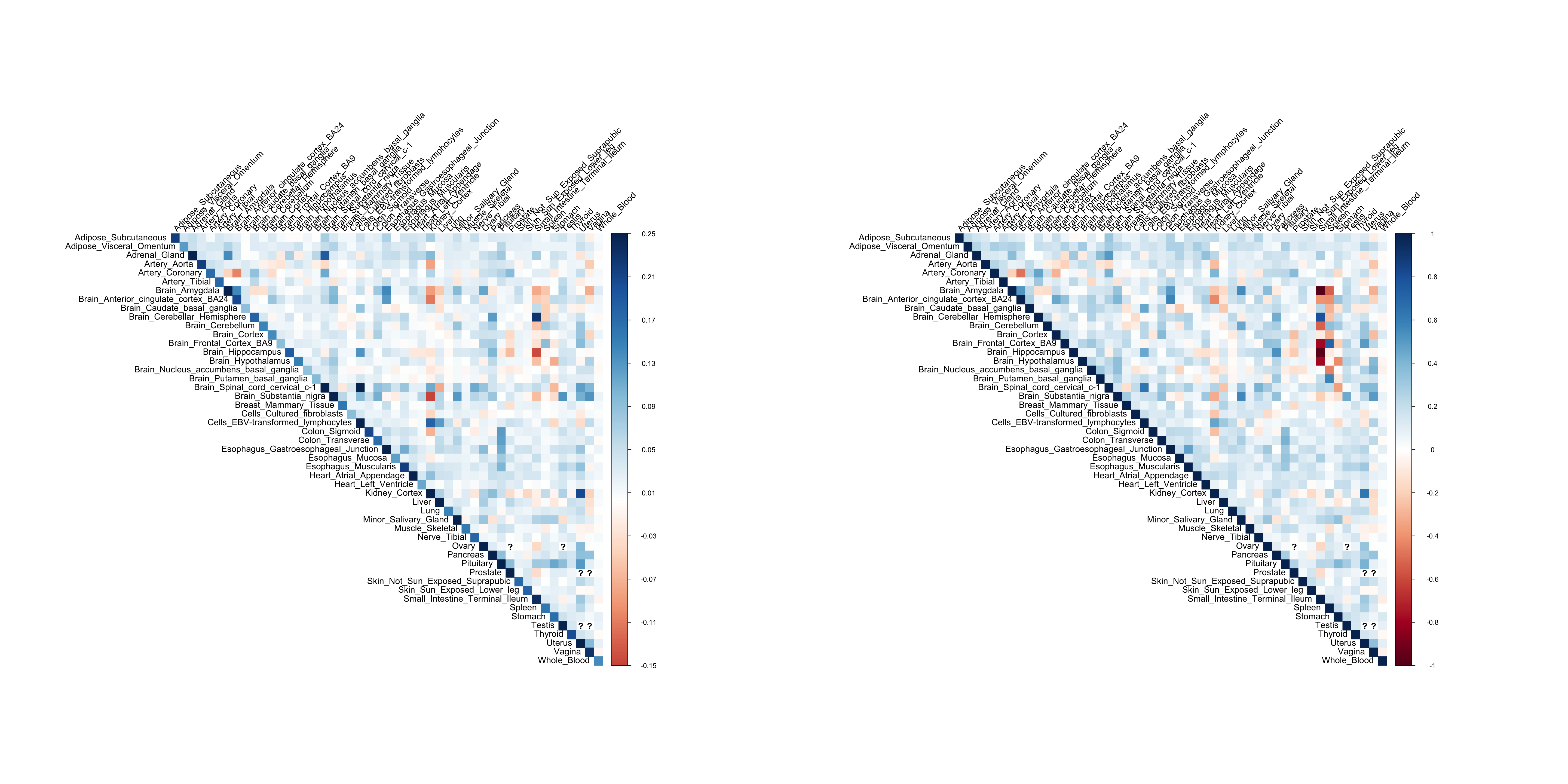
The covarince/correlation matrix of Y using FLASH:
colnames(resid_Y) = rownames(resid_Y) = colnames(Y)
par(mfrow=c(1,2))
corrplot(resid_Y, method='color', type='upper', tl.col="black", tl.srt=45, is.corr = FALSE)
corrplot(cov2cor(resid_Y), method='color', type='upper', tl.col="black", tl.srt=45, is.corr = TRUE)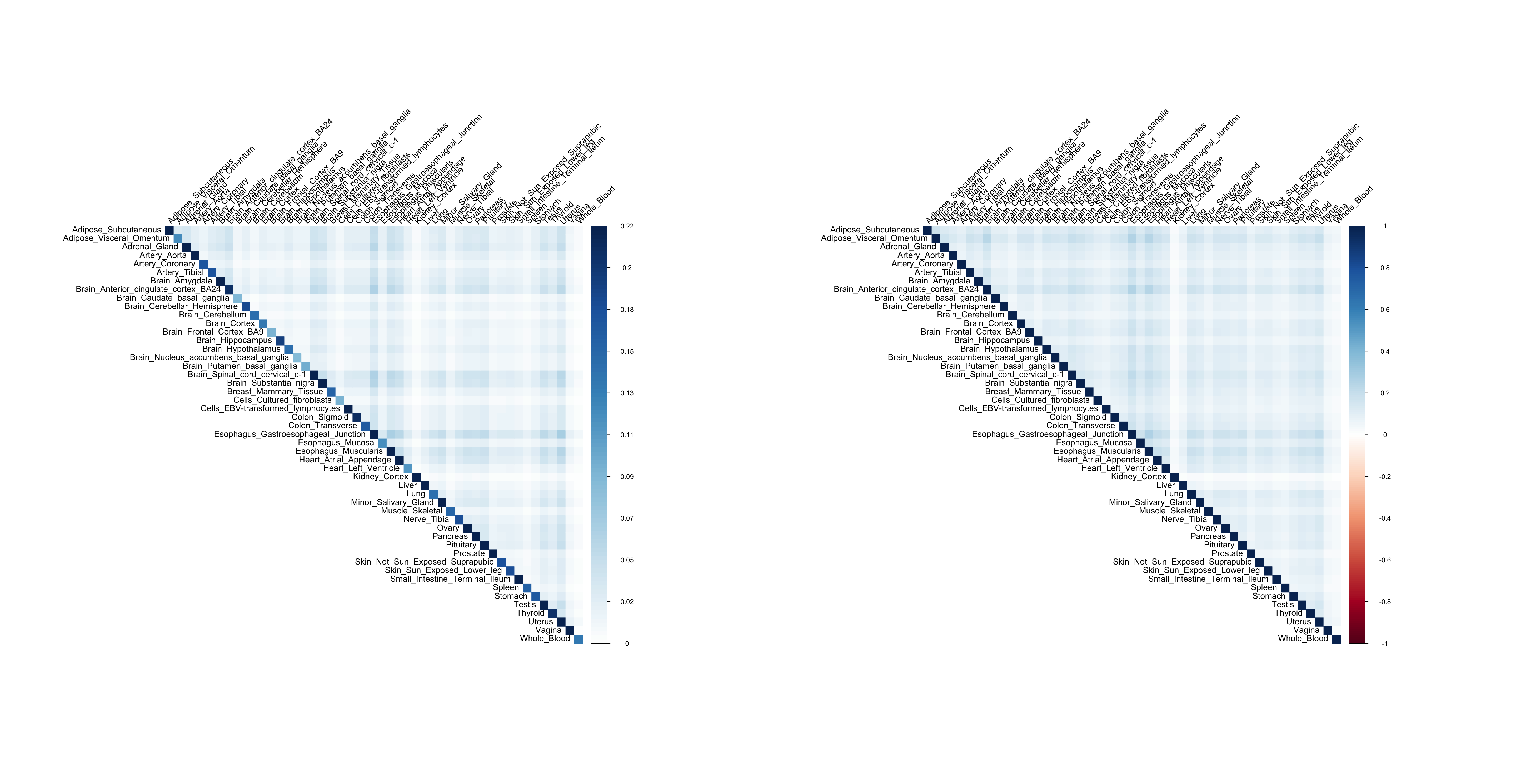
Models with L = 10
We fit 3 models with L = 10:
model with exact computation;
model with approximate computation;
model with approximate computation using diagonal residual variance, which is equivalent to exact computation with diagonal residual variance.
stime <- proc.time()
res <- mmbr::msusie(X, Y, prior_variance=prior, residual_variance=resid_Y, approximate=FALSE, compute_objective = T)
etime <- proc.time()
time_res <- etime - stime
saveRDS(list(result = res, result_time = time_res), 'output/GTExprofile_res_elbo.rds')
rm(res)

stime <- proc.time()
res_approx <- mmbr::msusie(X, Y, prior_variance=prior, residual_variance=resid_Y, approximate=TRUE, compute_objective = T)
etime <- proc.time()
time_res_approx <- etime - stime
saveRDS(list(result = res_approx, result_time = time_res_approx), 'output/GTExprofile_resapprox_elbo.rds')
rm(res_approx)

stime <- proc.time()
res_approx_diag <- mmbr::msusie(X, Y, prior_variance=prior, residual_variance=diag(diag(resid_Y)), approximate=TRUE, compute_objective = T)
etime <- proc.time()
time_res_approx_diag <- etime - stime
saveRDS(list(result = res_approx_diag, result_time = time_res_approx_diag), 'output/GTExprofile_resapproxdiag_elbo.rds')
rm(res_approx_diag)
Load models:
library(mmbr)Loading required package: mashrLoading required package: ashrLoading required package: susieRres1 = readRDS('output/GTExprofile_res_elbo.rds')
res2 = readRDS('output/GTExprofile_resapprox_elbo.rds')
res3 = readRDS('output/GTExprofile_resapproxdiag_elbo.rds')Model 1 credible sets:
susie_plot(res1$result, y='PIP', main=paste0('dense V, exact, ELBO=',round(res1$result$elbo[res1$result$niter], 2))) Model 2 credible sets:
susie_plot(res2$result, y='PIP', main=paste0('dense V, approx, ELBO=', round(res2$result$elbo[res2$result$niter], 2)))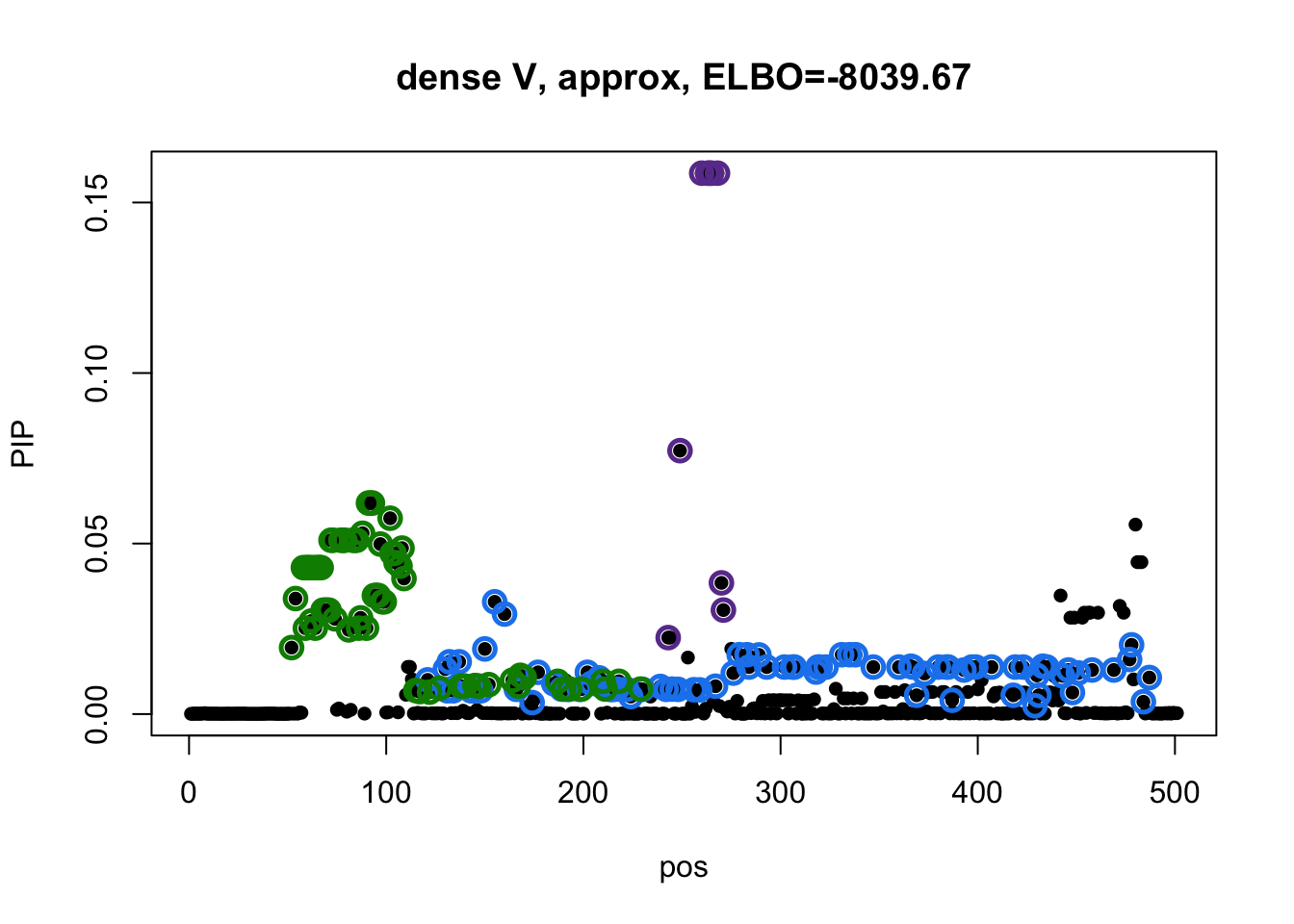 Model 3 credible sets:
susie_plot(res3$result, y='PIP', main=paste0('diagonal V, ELBO=', round(res3$result$elbo[res3$result$niter], 2)))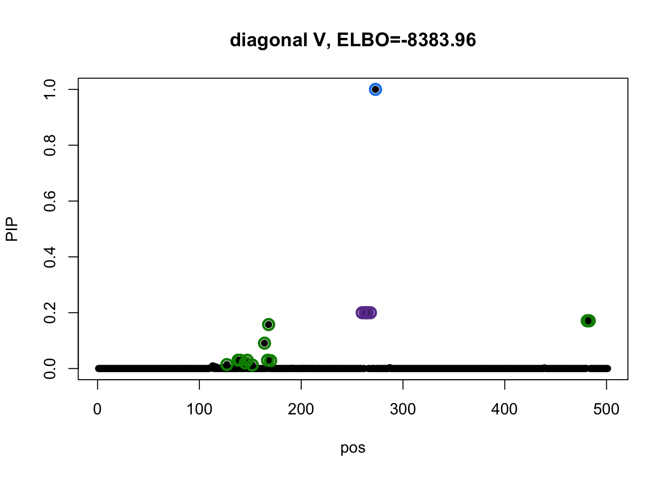
There is no overlapping between CSs. The blue CS in model 3 does not included in CSs from model 1 and 2.
| Total Time | Algorithm Time | # iterations | |
|---|---|---|---|
| model 1 | 1008.105 | 753.656 | 15 |
| model 2 | 724.233 | 701.838 | 15 |
| model 3 | 2184.959 | 2163.417 | 56 |
p = mmbr::mmbr_plot(res1$result)
pdf('docs/assets/GRExProfile/GTExprofile_res_elbo.pdf', width = 60, height = 15)
print(p$plot)
dev.off()p = mmbr::mmbr_plot(res2$result)
pdf('docs/assets/GRExProfile/GTExprofile_resapprox_elbo.pdf', width = 60, height = 15)
print(p$plot)
dev.off()p = mmbr::mmbr_plot(res3$result)
pdf('docs/assets/GRExProfile/GTExprofile_resapproxdiag_elbo.pdf', width = 5, height = 15)
print(p$plot)
dev.off()Models with L = 3
stime <- proc.time()
res <- mmbr::msusie(X, Y, prior_variance=prior, residual_variance=resid_Y, approximate=FALSE, L=3, compute_objective = T)
etime <- proc.time()
time_res <- etime - stime
saveRDS(list(result = res, result_time = time_res), 'output/GTExprofile_resL3_elbo.rds')

stime <- proc.time()
res_approx <- mmbr::msusie(X, Y, prior_variance=prior, residual_variance=resid_Y, approximate=TRUE, L=3, compute_objective = T)
etime <- proc.time()
time_res_approx <- etime - stime
saveRDS(list(result = res_approx, result_time = time_res_approx), 'output/GTExprofile_resapproxL3_elbo.rds')

stime <- proc.time()
res_approx_diag <- mmbr::msusie(X, Y, prior_variance=prior, residual_variance=diag(diag(resid_Y)), approximate=TRUE, L=3, compute_objective = T)
etime <- proc.time()
time_res_approx_diag <- etime - stime
saveRDS(list(result = res_approx_diag, result_time = time_res_approx_diag), 'output/GTExprofile_resapproxdiagL3_elbo.rds')
res1_L3 = readRDS('output/GTExprofile_resL3_elbo.rds')
res2_L3 = readRDS('output/GTExprofile_resapproxL3_elbo.rds')
res3_L3 = readRDS('output/GTExprofile_resapproxdiagL3_elbo.rds')Model 1 credible sets:
susie_plot(res1_L3$result, y='PIP', main=paste0('dense V, exact, ELBO=', round(res1_L3$result$elbo[res1_L3$result$niter], 2)))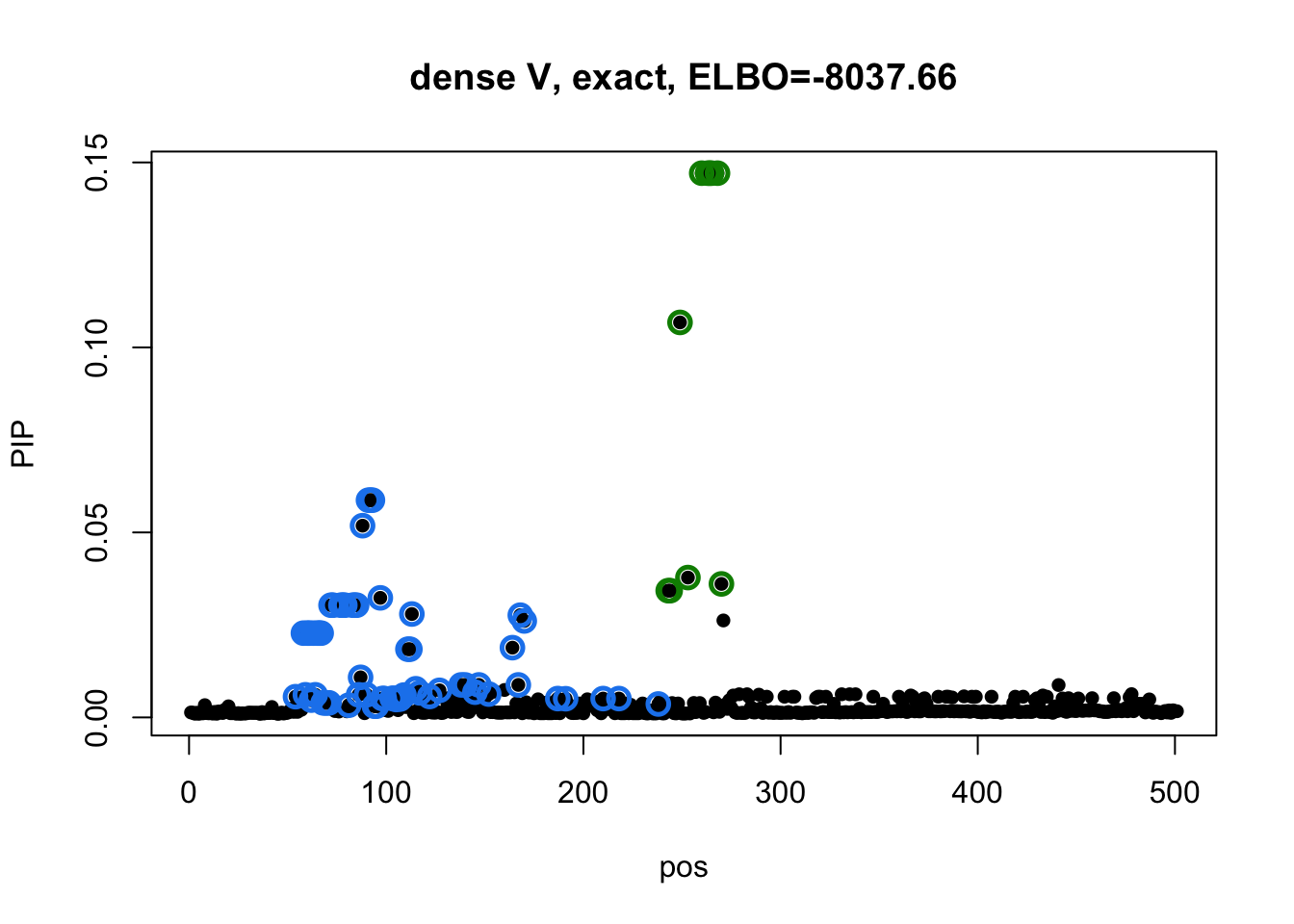 Model 2 credible sets:
susie_plot(res2_L3$result, y='PIP', main=paste0('dense V, approx, ELBO=', round(res2_L3$result$elbo[res2_L3$result$niter], 2)))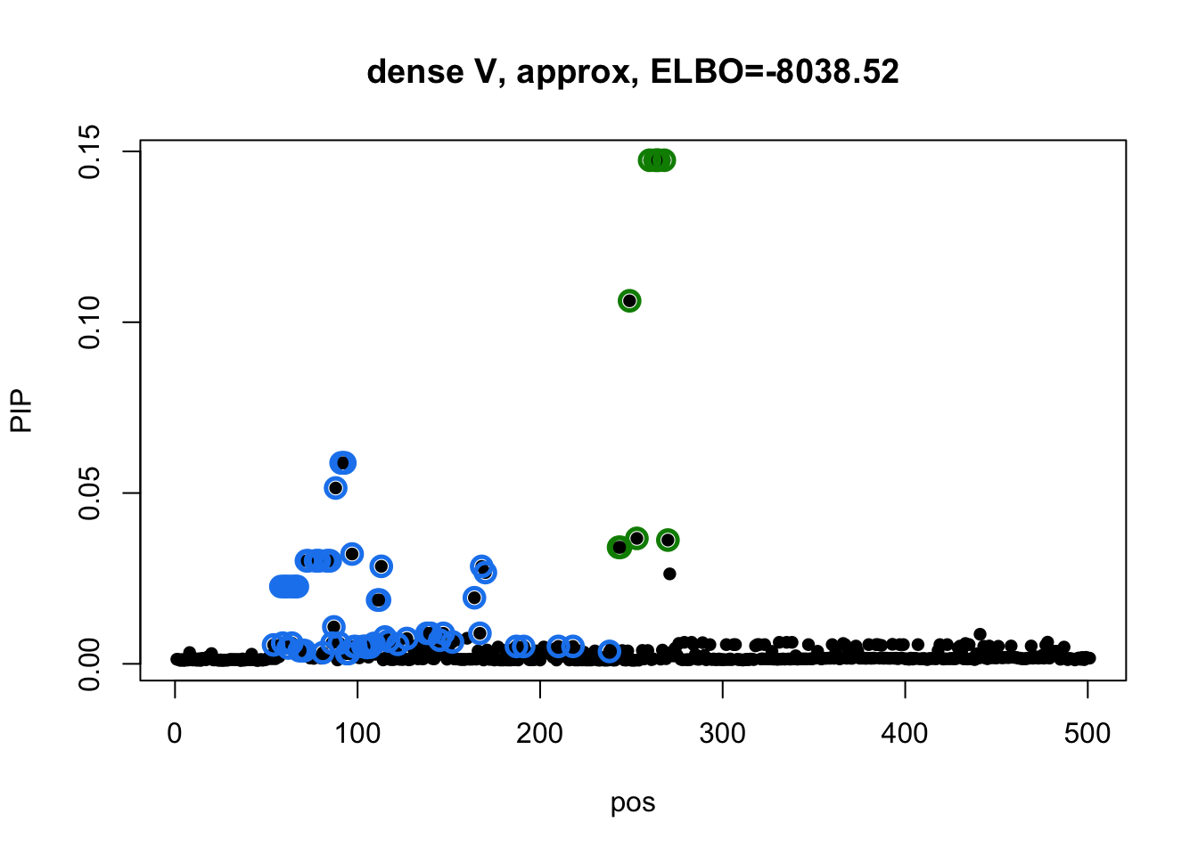 Model 3 credible sets:
susie_plot(res3_L3$result, y='PIP', main=paste0('diagonal V, ELBO=', round(res3_L3$result$elbo[res3_L3$result$niter], 2)))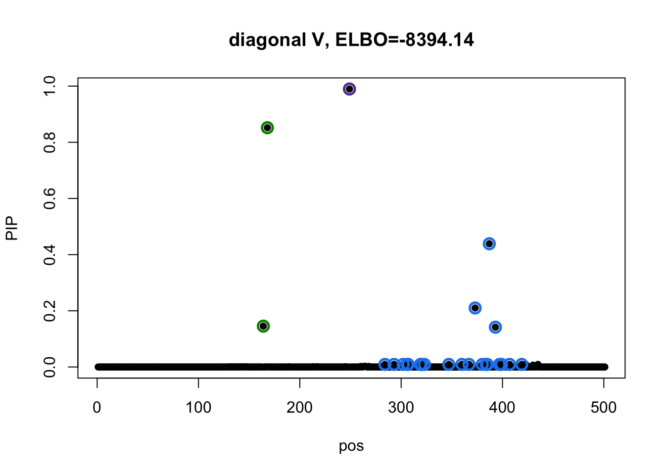
| Total Time | Algorithm Time | # iterations | |
|---|---|---|---|
| model 1 | 692.535 | 449.446 | 25 |
| model 2 | 502.582 | 482.78 | 25 |
| model 3 | 569.317 | 540.502 | 25 |
p = mmbr::mmbr_plot(res1_L3$result)
pdf('docs/assets/GRExProfile/GTExprofile_resL3_elbo.pdf', width = 17, height = 15)
print(p$plot)
dev.off()Models with L = 1
stime <- proc.time()
res <- mmbr::msusie(X, Y, prior_variance=prior, residual_variance=resid_Y, approximate=FALSE, L=1, compute_objective = T)
etime <- proc.time()
time_res <- etime - stime
saveRDS(list(result = res, result_time = time_res), 'output/GTExprofile_resL1_elbo.rds')

stime <- proc.time()
res_approx <- mmbr::msusie(X, Y, prior_variance=prior, residual_variance=resid_Y, approximate=TRUE, L=1, compute_objective = T)
etime <- proc.time()
time_res_approx <- etime - stime
saveRDS(list(result = res_approx, result_time = time_res_approx), 'output/GTExprofile_resapproxL1_elbo.rds')

stime <- proc.time()
res_approx_diag <- mmbr::msusie(X, Y, prior_variance=prior, residual_variance=diag(diag(resid_Y)), approximate=TRUE, L=1, compute_objective = T)
etime <- proc.time()
time_res_approx_diag <- etime - stime
saveRDS(list(result = res_approx_diag, result_time = time_res_approx_diag), 'output/GTExprofile_resapproxdiagL1_elbo.rds')
res1_L1 = readRDS('output/GTExprofile_resL1_elbo.rds')
res2_L1 = readRDS('output/GTExprofile_resapproxL1_elbo.rds')
res3_L1 = readRDS('output/GTExprofile_resapproxdiagL1_elbo.rds')Model 1 credible sets:
susie_plot(res1_L1$result, y='PIP', main=paste0('dense V, exact, ELBO=', round(res1_L1$result$elbo[res1_L1$result$niter], 2))) Model 2 credible sets:
susie_plot(res2_L1$result, y='PIP', main=paste0('dense V, approx, ELBO=', round(res2_L1$result$elbo[res2_L1$result$niter], 2)))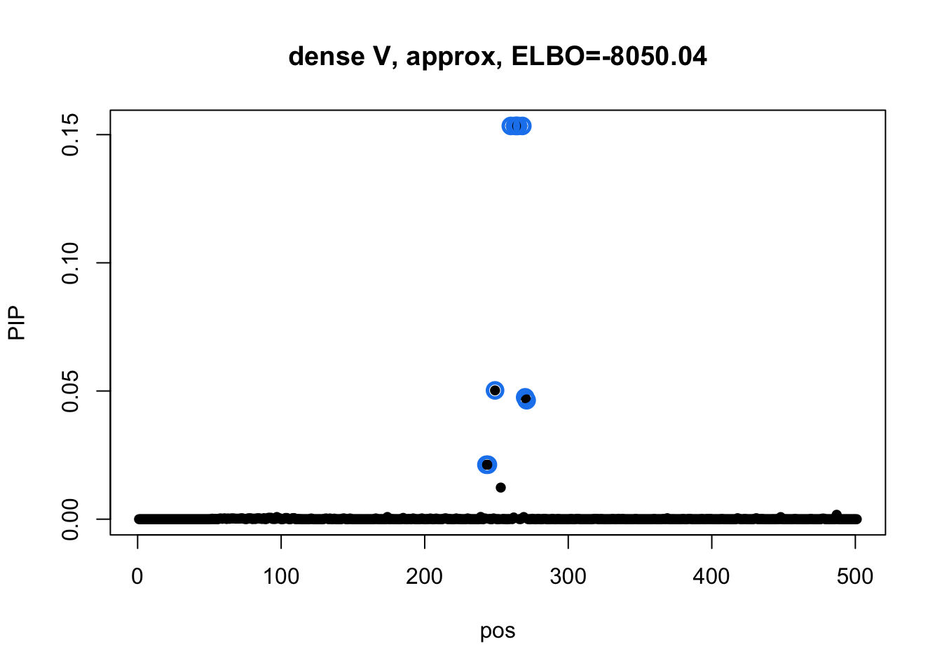 Model 3 credible sets:
susie_plot(res3_L1$result, y='PIP', main=paste0('diagonal V, ELBO=', round(res3_L1$result$elbo[res3_L1$result$niter], 2)))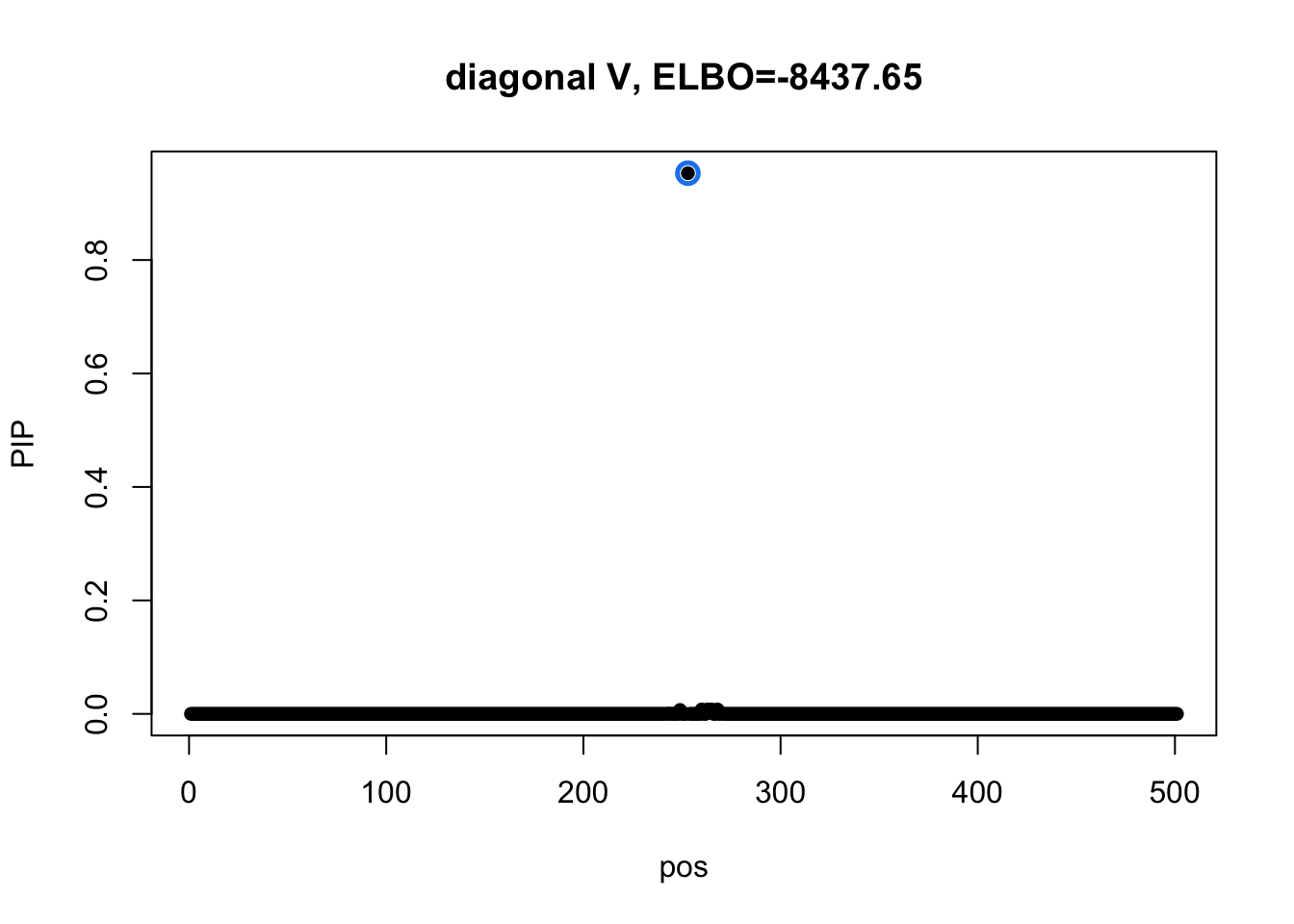
The CS from model 3 does not overlap any CSs from model 1.
sessionInfo()R version 3.6.3 (2020-02-29)
Platform: x86_64-apple-darwin15.6.0 (64-bit)
Running under: macOS Catalina 10.15.7
Matrix products: default
BLAS: /Library/Frameworks/R.framework/Versions/3.6/Resources/lib/libRblas.0.dylib
LAPACK: /Library/Frameworks/R.framework/Versions/3.6/Resources/lib/libRlapack.dylib
locale:
[1] en_US.UTF-8/en_US.UTF-8/en_US.UTF-8/C/en_US.UTF-8/en_US.UTF-8
attached base packages:
[1] stats graphics grDevices utils datasets methods base
other attached packages:
[1] mmbr_0.0.1.0305 susieR_0.9.26 mashr_0.2.40 ashr_2.2-51
[5] corrplot_0.84 workflowr_1.6.2
loaded via a namespace (and not attached):
[1] progress_1.2.2 tidyselect_1.1.0 xfun_0.19 purrr_0.3.4
[5] lattice_0.20-41 colorspace_1.4-1 vctrs_0.3.4 generics_0.1.0
[9] htmltools_0.5.0 yaml_2.2.1 rlang_0.4.8 mixsqp_0.3-46
[13] later_1.1.0.1 pillar_1.4.6 glue_1.4.2 plyr_1.8.6
[17] matrixStats_0.57.0 lifecycle_0.2.0 stringr_1.4.0 munsell_0.5.0
[21] gtable_0.3.0 flashier_0.2.7 mvtnorm_1.1-1 evaluate_0.14
[25] knitr_1.30 httpuv_1.5.4 invgamma_1.1 parallel_3.6.3
[29] irlba_2.3.3 Rcpp_1.0.5 promises_1.1.1 backports_1.2.0
[33] scales_1.1.1 rmeta_3.0 truncnorm_1.0-8 abind_1.4-5
[37] fs_1.5.0 ggplot2_3.3.2 hms_0.5.3 digest_0.6.27
[41] stringi_1.5.3 dplyr_1.0.2 ebnm_0.1-24 grid_3.6.3
[45] rprojroot_1.3-2 tools_3.6.3 magrittr_1.5 tibble_3.0.4
[49] crayon_1.3.4 whisker_0.4 pkgconfig_2.0.3 ellipsis_0.3.1
[53] Matrix_1.2-18 SQUAREM_2020.5 prettyunits_1.1.1 assertthat_0.2.1
[57] reshape_0.8.8 rmarkdown_2.5 rstudioapi_0.11 R6_2.5.0
[61] git2r_0.27.1 compiler_3.6.3