Introduction

This vignette is designed to describe some more advanced use of flash. Most users should start with the flash_intro.html vignette.

The interface described may change as we develop flashr.

Simulate Data

We start by simulating some data to provide an example:

library(flashr)
set.seed(1)
n = 100
p = 500
k = 7
LL = matrix(rnorm(n*k),nrow=n)
FF = matrix(rnorm(p*k),nrow=p)
Y = LL %*% t(FF) + rnorm(n*p)

Setting up data

For anything beyond the simplest usage, you should start your analysis by setting up the data in what we will call a “flash data object”. This is essentially simply an n by p matrix, but with meta-data to allow flash functions to deal properly with missing values etc. (This framework also makes it easier for future extensions to pass more information in as data; e.g. maybe variances also associated with the matrix).

data = flash_set_data(Y)

Initializing a factor model

Second, we need to initialize a factor model - essentially a set of factors and loadings. We call this a “flash fit object”, although at this point it is not actually fit to the data (this is the next step!) There are several ways to do this, using functions of the form flash_add_xxx. They are called this because they can add factors to an existing flash fit object—by providing a value for the argument f_init—so you can build up a flash fit object bit-by-bit. Here we have no existing flash fit object, so we do not specify f_init, and in this case these functions create a new fit object.

For illustration we show flash_add_factors_from_data. This essentially runs softImpute (soft-thresholded singular value decomposition) on the data to obtain an initial set of factors and loadings. We have to choose a number of factors to initialize with. (Factors can be dropped out during the fit so ideally this should be a larger number than we think we actually need; but at the same time more factors mean more computation, so you might start with a moderate number, and then try increasing later if the data seem to warrant it.)

f = flash_add_factors_from_data(data,K=10)

Refining/fitting a factor model

Once you have initialized a flash fit object, you can improve the fit using flash_backfit. (If you want to see how the fit is progressing, set verbose=TRUE here.)

f = flash_backfit(data,f,verbose=FALSE)

Extracting information

Having fit the model we might want to extract the fitted factors and loadings. You can do that using functions like flash_get_ldf to get the standardized loadings, factors and weights. Also flash_get_lf gets the product (LDF’). And flash_get_objective will return the measure of goodness-of-fit achieved (the variational lower bound, F). This can be helpful for comparing multiple fits to the same data.

plot(flash_get_lf(f), LL %*% t(FF),
     main="compare fitted values with true LF'")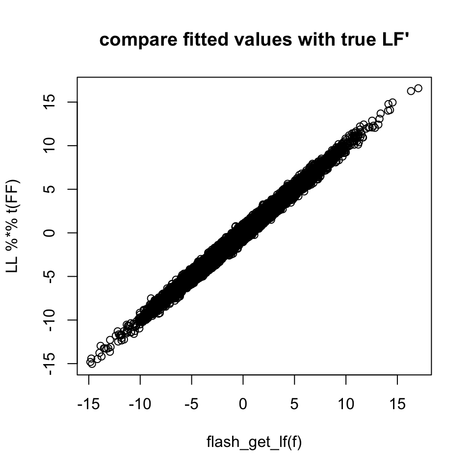

flash_get_ldf(f)$d
# [1] 303.3382 264.0119 242.3772 217.6895 208.5868 205.8112 183.3776
flash_get_objective(data,f)
# [1] -81253.75

Greedy addition of factors

The way we did it above was to add all the factors at once and then optimize. An alternative is to add one at a time, and optimize each in turn. This is accomplished using flash_add_greedy. This will keep adding factors until they no longer improve the fit, so you need to specify a maximum number to consider.

f_greedy = flash_add_greedy(data,Kmax=10)
# fitting factor/loading 1
# fitting factor/loading 2
# fitting factor/loading 3
# fitting factor/loading 4
# fitting factor/loading 5
# fitting factor/loading 6
# fitting factor/loading 7
# fitting factor/loading 8
flash_get_ldf(f_greedy)$d
# [1] 292.3761 253.6873 233.4289 210.8591 204.2400 203.0717 182.1317
flash_get_objective(data,f_greedy)
# [1] -84068.31

After adding factors in this way you can use backfitting to try to further improve the fit. In our experience, for different datasets, sometimes this provides a better fit than initializing all at once (as in f above), sometimes worse.

f_greedy_bf = flash_backfit(data,f_greedy)
flash_get_ldf(f_greedy_bf)$d
# [1] 303.7844 263.2466 241.8200 217.4748 209.0290 206.0587 183.2006
flash_get_objective(data,f_greedy_bf)
# [1] -81264.89
flash_get_objective(data,f)
# [1] -81253.75

Setting loadings and factors directly

In simulation experiments it might be useful to initialize the loadings and factors to the “truth” to see how it affects the convergence.

f_true = flash_add_lf(data, LL=LL, FF=FF)
f_cheat = flash_backfit(data,f_true)
flash_get_ldf(f_cheat)$d
# [1] 208.6823 214.9714 250.2059 213.0661 284.4945 221.1514 236.8675
flash_get_objective(data,f_cheat)
# [1] -81306.46

Unexpectedly (to me) the objective achieved from this initialization is lower than those from the greedy initialization. However, the results are pretty similar in terms of mean squared error (MSE). Notice that backfitting improved MSE vs greedy.

mean((flash_get_lf(f_cheat) - LL %*% t(FF))^2)
# [1] 0.08423822
mean((flash_get_lf(f_greedy_bf) - LL %*% t(FF))^2)
# [1] 0.08411568
mean((flash_get_lf(f) - LL %*% t(FF))^2)
# [1] 0.08426771
mean((flash_get_lf(f_greedy) - LL %*% t(FF))^2)
# [1] 0.09737634

Setting the function used to solve the EBNM problem

The flash algorithm involves iteratively applying a function that solves the “Empirical Bayes normal means” (EBNM) problem. See Wang and Stephens (2017) for more details on this. The flashr package provides two functions to do this: ebnm_pn, which uses a point-normal prior from the ebnm package, and ebnm_ash which provides an interface to functions in the ashr package.

In principle the ebnm_ash function fits a more flexible model, so might be preferred. However, in the paper we generally found the two methods give similar average performance, and ebnm_pn is (currently) faster, and so this is the default.

f_greedy_ash = flash_add_greedy(data,Kmax=10,ebnm_fn = ebnm_ash)
# fitting factor/loading 1
# fitting factor/loading 2
# fitting factor/loading 3
# fitting factor/loading 4
# fitting factor/loading 5
# fitting factor/loading 6
# fitting factor/loading 7
# fitting factor/loading 8
flash_get_objective(data,f_greedy_ash)
# [1] -84075.06

Fixed factors or loadings

Sometimes you might want to include a “fixed” factor or loading in the analysis. For example, maybe you have a covariate you are interested in the effect of. Or you want to include a mean term in the rows or columns. You can add such “fixed” factors using flash_add_fixed_l or flash_add_fixed_f. Fixed loadings will not be updated during a subsequent fit, but their corresponding factors will be updated. Similarly, fixed factors will not be updated, but their loadings will be. (Missing values, NA, in a fixed loading or factor are allowed and will be updated during a fit.)

For example, the following creates a flash fit object with a fixed intercept loading. (So when fit it will estimate a corresponding factor, which should be interpreted as a column-specific mean.) Then it adds 10 data-based factors and loadings, and then it fits the model. Note how the first loading (the mean) does not change during the fit. (Notice also that the corresponding factor is 0—correct since we did not add a non-zero mean to the simulation.)

f = flash_add_fixed_l(data,LL = cbind(rep(1,n)))
f = flash_add_factors_from_data(data,K=10,f_init=f)
f = flash_backfit(data,f)
flash_get_k(f) #tells you how many factors f has
# [1] 11
head(flash_get_ldf(f,1,drop_zero_factors = FALSE)$l)
#      [,1]
# [1,]  0.1
# [2,]  0.1
# [3,]  0.1
# [4,]  0.1
# [5,]  0.1
# [6,]  0.1
# Note this is 0 as the factor has no weight
flash_get_ldf(f,1,drop_zero_factors = FALSE)$d
# [1] 0