A closer look at some results on the 68K PBMC data
Peter Carbonetto
Last updated: 2025-07-01
Checks: 7 0
Knit directory:
fastTopics-experiments/analysis/
This reproducible R Markdown analysis was created with workflowr (version 1.7.1). The Checks tab describes the reproducibility checks that were applied when the results were created. The Past versions tab lists the development history.
Great! Since the R Markdown file has been committed to the Git repository, you know the exact version of the code that produced these results.
Great job! The global environment was empty. Objects defined in the global environment can affect the analysis in your R Markdown file in unknown ways. For reproduciblity it’s best to always run the code in an empty environment.
The command set.seed(1) was run prior to running the
code in the R Markdown file. Setting a seed ensures that any results
that rely on randomness, e.g. subsampling or permutations, are
reproducible.
Great job! Recording the operating system, R version, and package versions is critical for reproducibility.
Nice! There were no cached chunks for this analysis, so you can be confident that you successfully produced the results during this run.
Great job! Using relative paths to the files within your workflowr project makes it easier to run your code on other machines.
Great! You are using Git for version control. Tracking code development and connecting the code version to the results is critical for reproducibility.
The results in this page were generated with repository version 9168f5d. See the Past versions tab to see a history of the changes made to the R Markdown and HTML files.
Note that you need to be careful to ensure that all relevant files for
the analysis have been committed to Git prior to generating the results
(you can use wflow_publish or
wflow_git_commit). workflowr only checks the R Markdown
file, but you know if there are other scripts or data files that it
depends on. Below is the status of the Git repository when the results
were generated:
Ignored files:
    Ignored:    analysis/.sos/
    Ignored:    data/20news-bydate/
    Ignored:    data/droplet.RData
    Ignored:    data/nips_1-17.mat
    Ignored:    data/pbmc_68k.RData
    Ignored:    output/droplet/fits-droplet.RData
    Ignored:    output/droplet/lda-droplet.RData
    Ignored:    output/newsgroups/de-newsgroups.RData
    Ignored:    output/newsgroups/fits-newsgroups.RData
    Ignored:    output/newsgroups/lda-newsgroups.RData
    Ignored:    output/newsgroups/rds/
    Ignored:    output/nips/fits-nips.RData
    Ignored:    output/nips/lda-nips.RData
    Ignored:    output/pbmc68k/rds/

Untracked files:
    Untracked:  analysis/lda-eb-newsgroups-em-k=10.rds
    Untracked:  analysis/lda-eb-newsgroups-scd-ex-k=10.rds
    Untracked:  analysis/lda-newsgroups-em-k=10.rds
    Untracked:  analysis/lda-newsgroups-scd-ex-k=10.rds
    Untracked:  analysis/maptpx-newsgroups-em-k=10.rds
    Untracked:  analysis/maptpx-newsgroups-scd-ex-k=10.rds
    Untracked:  analysis/mcf7_cache/
    Untracked:  plots/
Note that any generated files, e.g. HTML, png, CSS, etc., are not included in this status report because it is ok for generated content to have uncommitted changes.
These are the previous versions of the repository in which changes were
made to the R Markdown (analysis/pbmc68k_more.Rmd) and HTML
(docs/pbmc68k_more.html) files. If you’ve configured a
remote Git repository (see ?wflow_git_remote), click on the
hyperlinks in the table below to view the files as they were in that
past version.
| File | Version | Author | Date | Message |
|---|---|---|---|---|
| Rmd | 9168f5d | Peter Carbonetto | 2025-07-01 | wflow_publish("pbmc68k_more.Rmd", verbose = T, view = F) |
| html | 399fc57 | Peter Carbonetto | 2024-08-13 | Built the pbmc68k_more workflowr page. |
| Rmd | e9a5583 | Peter Carbonetto | 2024-08-13 | workflowr::wflow_publish("pbmc68k_more.Rmd", verbose = TRUE) |
Here we take a closer look at some of the results on the 68K PBMC data.
Load the packages used in this analysis.
library(Matrix)
library(topicmodels)
library(fastTopics)
library(ggplot2)
library(cowplot)
Load the 68K PBMC data.
load("../data/pbmc_68k.RData")
rm(counts)
Load the topic models fit using the EM and CD algorithms
fit1 <- readRDS("../output/pbmc68k/rds/fit-pbmc68k-em-k=7.rds")$fit
fit2 <- readRDS("../output/pbmc68k/rds/fit-pbmc68k-scd-ex-k=7.rds")$fit
fit1 <- poisson2multinom(fit1)
fit2 <- poisson2multinom(fit2)
and the LDA fits initialized using the EM and CD estimates:
lda1 <- readRDS("../output/pbmc68k/rds/lda-pbmc68k-em-k=7.rds")$lda
lda2 <- readRDS("../output/pbmc68k/rds/lda-pbmc68k-scd-ex-k=7.rds")$lda
The MLEs and the approximate posterior estimates from LDA turn out to be very similar to each other, so there is really no need to examine both. Here we’ll focus on the MLEs:
cor(as.vector(fit1$L),as.vector(lda1@gamma))
cor(as.vector(fit2$L),as.vector(lda2@gamma))
# [1] 0.9471059
# [1] 0.9654844
Let’s now examine the results using Structure plots. Here are the EM estimates:
L <- fit2$L
n <- nrow(L)
clusters <- rep("T cells",n)
names(clusters) <- rownames(fit2$L)
clusters[L[,3] > 0.4] <- "NK cells"
clusters[L[,1] > 0.3] <- "myeloid"
clusters[L[,5] > 0.2] <- "B cells"
clusters[L[,2] > 0.9] <- "Megakaryocytes"
clusters <- factor(clusters,
                   c("Megakaryocytes","myeloid","B cells","NK cells",
                     "T cells"))
n    <- nrow(fit1$L)
rows <- c(sample(which(clusters == "T cells"),400),
          sample(which(clusters != "T cells"),650))
fit1 <- select_loadings(fit1,rows)
fit2 <- select_loadings(fit2,rows)
k <- 7
topic_colors <- c("#a6cee3","#1f78b4","#b2df8a","#33a02c","#fb9a99",
                  "#e31a1c","#fdbf6f")
set.seed(1)
p1 <- structure_plot(fit1,grouping = clusters[rows],topics = 1:7,
                     colors = topic_colors,gap = 10)
  ggtitle("EM without extrapolation") +
  theme(plot.title = element_text(face = "plain",size = 10))
p1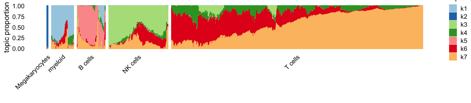
| Version | Author | Date |
|---|---|---|
| 399fc57 | Peter Carbonetto | 2024-08-13 |
And here are the CD estimates:
p2 <- structure_plot(fit2,grouping = clusters[rows],topics = 1:7,
                     colors = topic_colors,gap = 10)
  ggtitle("CD with extrapolation") +
  theme(plot.title = element_text(face = "plain",size = 10))
p2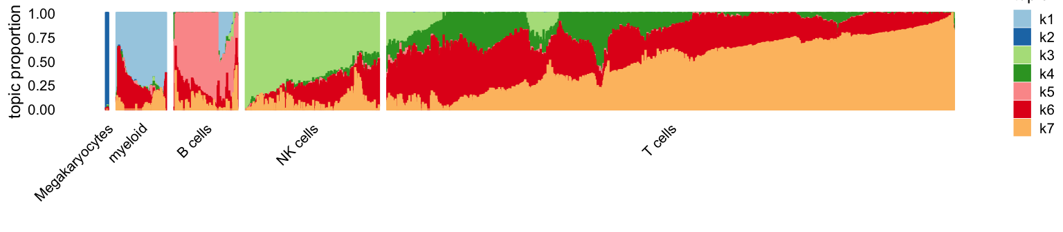
| Version | Author | Date |
|---|---|---|
| 399fc57 | Peter Carbonetto | 2024-08-13 |
The most striking difference is the greater promenance of topic 6 (red).
Let’s now extract some “driving genes” for a few selected topics by taking genes that are at higher expression in the given topic compared to the other topics. For example, some of the top driving genes for topic 1 suggest myeloid cells (e.g., S100A8, S100A9):
k <- 1
dat <- data.frame(gene = genes$symbol,
                  f0 = apply(fit2$F[,-k],1,max),
                  f1 = fit1$F[,k],
                  f2 = fit2$F[,k])
dat <- transform(dat,lfc = log2(f2/f0))
subset(dat,lfc > 4 & f2 > 0.001)
#                     gene           f0          f1          f2       lfc
# ENSG00000163220   S100A9 3.658675e-18 0.004101862 0.004143481 50.008444
# ENSG00000143546   S100A8 3.658675e-18 0.002850460 0.002879382 49.483359
# ENSG00000204482     LST1 1.225331e-04 0.005464021 0.005506292  5.489838
# ENSG00000204472     AIF1 1.647450e-04 0.006086946 0.006151222  5.222566
# ENSG00000126759      CFP 2.860184e-05 0.001149577 0.001162555  5.345047
# ENSG00000085265     FCN1 3.658675e-18 0.001976919 0.001996978 48.955418
# ENSG00000090382      LYZ 3.658675e-18 0.006543255 0.006609647 50.682173
# ENSG00000197249 SERPINA1 4.840894e-06 0.001345175 0.001358822  8.132868
# ENSG00000197766      CFD 3.658675e-18 0.001736280 0.001753897 48.768164
# ENSG00000216490    IFI30 1.338963e-05 0.001119325 0.001131379  6.400823
# ENSG00000025708     TYMP 1.146609e-04 0.001830871 0.001872341  4.029397
The top driving genes for topic 5 suggest B cells (e.g., CD79A, CD19):
k <- 5
dat <- data.frame(gene = genes$symbol,
                  f0 = apply(fit2$F[,-k],1,max),
                  f1 = fit1$F[,k],
                  f2 = fit2$F[,k])
dat <- transform(dat,lfc = log2(f2/f0))
subset(dat,lfc > 10 & f2 > 0.0001)
#                       gene           f0           f1           f2      lfc
# ENSG00000132185      FCRLA 3.658675e-18 0.0001962006 0.0001960767 45.60709
# ENSG00000163687   DNASE1L3 3.658675e-18 0.0001064082 0.0001063410 44.72437
# ENSG00000132465        IGJ 3.658675e-18 0.0006496942 0.0006492841 47.33452
# ENSG00000170476       MZB1 3.658675e-18 0.0005379152 0.0005375756 47.06214
# ENSG00000241106    HLA-DOB 3.658675e-18 0.0002418521 0.0002416994 45.90889
# ENSG00000168081       PNOC 3.658675e-18 0.0001780743 0.0001779618 45.46724
# ENSG00000184709     LRRC26 3.658675e-18 0.0001030515 0.0001029864 44.67813
# ENSG00000095585       BLNK 3.658675e-18 0.0001270521 0.0001269718 44.98018
# ENSG00000156738      MS4A1 3.658675e-18 0.0008338106 0.0008332842 47.69448
# ENSG00000100721      TCL1A 3.658675e-18 0.0012611217 0.0012603256 48.29140
# ENSG00000253701 AL928768.3 3.658675e-18 0.0003640369 0.0003638071 46.49885
# ENSG00000247982  LINC00926 3.658675e-18 0.0003821632 0.0003819219 46.56895
# ENSG00000177455       CD19 3.658675e-18 0.0001617942 0.0001616920 45.32892
# ENSG00000104921      FCER2 3.658675e-18 0.0002896854 0.0002895025 46.16925
# ENSG00000105369      CD79A 3.658675e-18 0.0028936650 0.0028918385 49.48959
# ENSG00000269404       SPIB 3.658675e-18 0.0003084831 0.0003082883 46.25995
# ENSG00000254709      IGLL5 3.658675e-18 0.0017324059 0.0017313124 48.74947
# ENSG00000128218     VPREB3 3.658675e-18 0.0003151965 0.0003149975 46.29101
# ENSG00000099958      DERL3 3.658675e-18 0.0001495421 0.0001494477 45.21531
The top driving genes for topic 3 suggest natural killer (NK) cells (e.g., NKG7, GNLY):
k <- 3
dat <- data.frame(gene = genes$symbol,
                  f0 = apply(fit2$F[,-k],1,max),
                  f1 = fit1$F[,k],
                  f2 = fit2$F[,k])
dat <- transform(dat,lfc = log2(f2/f0))
subset(dat,lfc > 4 & f2 > 0.001)
#                   gene           f0          f1          f2       lfc
# ENSG00000115523   GNLY 3.658675e-18 0.015808531 0.015202766 51.883862
# ENSG00000137441 FGFBP2 3.658675e-18 0.001855115 0.001784029 48.792739
# ENSG00000145649   GZMA 1.180503e-04 0.003478113 0.003409834  4.852228
# ENSG00000169583  CLIC3 3.184806e-05 0.001393214 0.001336228  5.390816
# ENSG00000180644   PRF1 2.631073e-05 0.001433384 0.001381024  5.713943
# ENSG00000100450   GZMH 3.658675e-18 0.002288307 0.002200621 49.095511
# ENSG00000100453   GZMB 3.658675e-18 0.003223107 0.003099601 49.589683
# ENSG00000077984   CST7 8.545444e-05 0.003252106 0.003141172  5.200003
# ENSG00000105374   NKG7 3.658675e-18 0.012121078 0.011656612 51.500677
Topic 2 is less clear, but perhaps relates to megakaryocytes (e.g., PF4):
k <- 2
dat <- data.frame(gene = genes$symbol,
                  f0 = apply(fit2$F[,-k],1,max),
                  f1 = fit1$F[,k],
                  f2 = fit2$F[,k])
dat <- transform(dat,lfc = log2(f2/f0))
subset(dat,lfc > 10 & f2 > 0.001)
#                       gene           f0          f1          f2      lfc
# ENSG00000171848       RRM2 8.244439e-19 0.001064246 0.001026667 50.14540
# ENSG00000187699    C2orf88 8.244439e-19 0.001076621 0.001038605 50.16207
# ENSG00000168497       SDPR 8.244439e-19 0.007816845 0.007540828 53.02215
# ENSG00000088726     TMEM40 8.244439e-19 0.001319995 0.001273385 50.45610
# ENSG00000169704        GP9 8.244439e-19 0.003316487 0.003199380 51.78522
# ENSG00000163737        PF4 8.244439e-19 0.011009582 0.010620828 53.51625
# ENSG00000163736       PPBP 8.244439e-19 0.033267996 0.032093286 55.11163
# ENSG00000113140      SPARC 8.244439e-19 0.003308237 0.003191421 51.78163
# ENSG00000124491      F13A1 8.244439e-19 0.001010377 0.001038604 50.16207
# ENSG00000180573  HIST1H2AC 8.244439e-19 0.010073211 0.009717520 53.38802
# ENSG00000124635  HIST1H2BJ 8.244439e-19 0.001187995 0.001146045 50.30409
# ENSG00000161911     TREML1 8.244439e-19 0.002804989 0.002705943 51.54356
# ENSG00000171611      PTCRA 8.244439e-19 0.004855106 0.004683670 52.33507
# ENSG00000223855 AC147651.3 8.244439e-19 0.001357120 0.001309199 50.49611
# ENSG00000127920      GNG11 8.244439e-19 0.009041965 0.008722688 53.23220
# ENSG00000120885        CLU 8.244439e-19 0.008353093 0.008058140 53.11788
# ENSG00000236304 AP001189.4 8.244439e-19 0.001538619 0.001484290 50.67720
# ENSG00000111644      ACRBP 8.244439e-19 0.004673607 0.004508579 52.28010
# ENSG00000165682     CLEC1B 8.244439e-19 0.001047746 0.001010749 50.12285
# ENSG00000102804    TSC22D1 8.244439e-19 0.003844485 0.003708733 51.99835
# ENSG00000166091      CMTM5 8.244439e-19 0.002664740 0.002570646 51.46956
# ENSG00000166803   KIAA0101 8.244439e-19 0.001355746 0.001679276 50.85527
# ENSG00000131153      GINS2 8.244439e-19 0.001187881 0.001146045 50.30409
# ENSG00000005961     ITGA2B 8.244439e-19 0.002495615 0.002407494 51.37496
# ENSG00000167900        TK1 8.244439e-19 0.001493244 0.001440516 50.63401
# ENSG00000176890       TYMS 8.244439e-19 0.001596369 0.001540000 50.73036
# ENSG00000101335       MYL9 8.244439e-19 0.002875114 0.002773592 51.57918
# ENSG00000101162      TUBB1 8.244439e-19 0.003959985 0.003820155 52.04106
# ENSG00000184113      CLDN5 8.244439e-19 0.001988242 0.001918036 51.04706
Topic 6, the topic that is most different between the EM and CD estimates, appears to be capturing a “baseline” expression level. This includes ribosomal protein genes, which account for a large fraction of the total expression in this data set, and don’t capture any “interesting” structure.
k <- 6
dat <- data.frame(gene = genes$symbol,
                  f0 = apply(fit2$F[,-k],1,max),
                  f1 = fit1$F[,k],
                  f2 = fit2$F[,k])
dat <- transform(dat,lfc = log2(f2/f0),r21 = f2/f1)
subset(dat,lfc > 0.5 & f2 > 0.005)
#                   gene          f0          f1          f2       lfc      r21
# ENSG00000142937   RPS8 0.006212607 0.007282610 0.009452406 0.6054827 1.297942
# ENSG00000171863   RPS7 0.005103906 0.006529843 0.007528874 0.5608325 1.152995
# ENSG00000143947 RPS27A 0.006723131 0.008274633 0.010216551 0.6037030 1.234683
# ENSG00000168028   RPSA 0.003996081 0.006059185 0.006866905 0.7810739 1.133305
# ENSG00000188846  RPL14 0.005299126 0.006768258 0.007777698 0.5535889 1.149143
# ENSG00000182899 RPL35A 0.004289314 0.004887549 0.006240801 0.5409843 1.276877
# ENSG00000163682   RPL9 0.005517871 0.006043094 0.007906552 0.5189369 1.308362
# ENSG00000109475  RPL34 0.006583338 0.007406409 0.009832636 0.5787590 1.327585
# ENSG00000164587  RPS14 0.009615048 0.011499182 0.015354971 0.6753398 1.335310
# ENSG00000231500  RPS18 0.009480947 0.014997337 0.018356074 0.9531545 1.223956
# ENSG00000198755 RPL10A 0.005820401 0.006879194 0.008766827 0.5909361 1.274397
# ENSG00000156508 EEF1A1 0.004581784 0.006090634 0.007081075 0.6280589 1.162617
# ENSG00000112306  RPS12 0.007329941 0.009894959 0.013415214 0.8719966 1.355762
# ENSG00000198034  RPS4X 0.011496567 0.014915339 0.017746177 0.6263052 1.189794
# ENSG00000147403  RPL10 0.014871444 0.021420213 0.024814561 0.7386422 1.158465
# ENSG00000137154   RPS6 0.013645329 0.016713112 0.021149907 0.6322442 1.265468
# ENSG00000136942  RPL35 0.003344397 0.004645911 0.005430991 0.6994693 1.168983
# ENSG00000197958  RPL12 0.006380061 0.007971636 0.009766431 0.6142612 1.225148
# ENSG00000177600  RPLP2 0.006496343 0.007591369 0.010241558 0.6567354 1.349106
# ENSG00000166441 RPL27A 0.004811566 0.006516915 0.007933225 0.7214009 1.217328
# ENSG00000149273   RPS3 0.010058599 0.015101867 0.018217486 0.8568946 1.206307
# ENSG00000118181  RPS25 0.004734571 0.005359617 0.006793787 0.5209821 1.267588
# ENSG00000089009   RPL6 0.005969072 0.007889148 0.009177513 0.6205967 1.163309
# ENSG00000089157  RPLP0 0.003910155 0.005630981 0.006419673 0.7152742 1.140063
# ENSG00000133112   TPT1 0.004401657 0.005584376 0.006232404 0.5017421 1.116043
# ENSG00000137818  RPLP1 0.007683192 0.009954931 0.011870655 0.6276218 1.192440
# ENSG00000140988   RPS2 0.016451406 0.024278162 0.029134934 0.8245392 1.200047
# ENSG00000167526  RPL13 0.018347801 0.024632966 0.031966430 0.8009505 1.297709
# ENSG00000161970  RPL26 0.004613366 0.006136206 0.007274305 0.6569896 1.185473
# ENSG00000198242 RPL23A 0.005460498 0.008053744 0.009302257 0.7685482 1.155023
# ENSG00000108298  RPL19 0.009078556 0.011152563 0.013661245 0.5895543 1.224942
# ENSG00000115268  RPS15 0.005863653 0.006905223 0.008340809 0.5083877 1.207899
# ENSG00000105640 RPL18A 0.009469537 0.011050546 0.013491073 0.5106392 1.220851
# ENSG00000105193  RPS16 0.004297136 0.005087433 0.006463933 0.5890368 1.270569
# ENSG00000105372  RPS19 0.007791512 0.011259541 0.014157993 0.8616415 1.257422
# ENSG00000063177  RPL18 0.005866878 0.007475159 0.009252083 0.6571851 1.237710
# ENSG00000142541 RPL13A 0.014060044 0.019979209 0.024286719 0.7885665 1.215600
# ENSG00000170889   RPS9 0.005723394 0.007022134 0.009275166 0.6965022 1.320847
# ENSG00000108107  RPL28 0.004654791 0.006365727 0.007340847 0.6572300 1.153183
# ENSG00000100316   RPL3 0.012288336 0.015768331 0.020156959 0.7139884 1.278319
sessionInfo()
# R version 4.3.3 (2024-02-29)
# Platform: aarch64-apple-darwin20 (64-bit)
# Running under: macOS 15.5
#
# Matrix products: default
# BLAS:   /Library/Frameworks/R.framework/Versions/4.3-arm64/Resources/lib/libRblas.0.dylib
# LAPACK: /Library/Frameworks/R.framework/Versions/4.3-arm64/Resources/lib/libRlapack.dylib;  LAPACK version 3.11.0
#
# locale:
# [1] en_US.UTF-8/en_US.UTF-8/en_US.UTF-8/C/en_US.UTF-8/en_US.UTF-8
#
# time zone: America/Chicago
# tzcode source: internal
#
# attached base packages:
# [1] stats     graphics  grDevices utils     datasets  methods   base
#
# other attached packages:
# [1] cowplot_1.1.3      ggplot2_3.5.0      fastTopics_0.7-25  topicmodels_0.2-16
# [5] Matrix_1.6-5
#
# loaded via a namespace (and not attached):
#  [1] tidyselect_1.2.1    viridisLite_0.4.2   dplyr_1.1.4
#  [4] farver_2.1.1        fastmap_1.1.1       lazyeval_0.2.2
#  [7] promises_1.2.1      digest_0.6.34       lifecycle_1.0.4
# [10] NLP_0.2-1           invgamma_1.1        magrittr_2.0.3
# [13] compiler_4.3.3      rlang_1.1.5         sass_0.4.9
# [16] progress_1.2.3      tools_4.3.3         utf8_1.2.4
# [19] yaml_2.3.8          data.table_1.17.4   knitr_1.45
# [22] prettyunits_1.2.0   labeling_0.4.3      htmlwidgets_1.6.4
# [25] plyr_1.8.9          xml2_1.3.6          Rtsne_0.17
# [28] workflowr_1.7.1     withr_3.0.2         purrr_1.0.2
# [31] grid_4.3.3          stats4_4.3.3        fansi_1.0.6
# [34] git2r_0.33.0        tm_0.7-13           colorspace_2.1-0
# [37] scales_1.3.0        gtools_3.9.5        cli_3.6.4
# [40] rmarkdown_2.26      crayon_1.5.2        ragg_1.2.7
# [43] generics_0.1.3      RcppParallel_5.1.10 httr_1.4.7
# [46] reshape2_1.4.4      pbapply_1.7-2       cachem_1.0.8
# [49] stringr_1.5.1       modeltools_0.2-23   parallel_4.3.3
# [52] vctrs_0.6.5         jsonlite_1.8.8      slam_0.1-50
# [55] hms_1.1.3           mixsqp_0.3-54       ggrepel_0.9.5
# [58] irlba_2.3.5.1       systemfonts_1.0.6   plotly_4.10.4
# [61] jquerylib_0.1.4     tidyr_1.3.1         glue_1.8.0
# [64] uwot_0.2.3          stringi_1.8.3       gtable_0.3.4
# [67] later_1.3.2         quadprog_1.5-8      munsell_0.5.0
# [70] tibble_3.2.1        pillar_1.9.0        htmltools_0.5.8.1
# [73] truncnorm_1.0-9     R6_2.5.1            textshaping_0.3.7
# [76] rprojroot_2.0.4     evaluate_1.0.3      lattice_0.22-5
# [79] highr_0.10          RhpcBLASctl_0.23-42 SQUAREM_2021.1
# [82] ashr_2.2-66         httpuv_1.6.14       bslib_0.6.1
# [85] Rcpp_1.0.12         whisker_0.4.1       xfun_0.42
# [88] fs_1.6.5            pkgconfig_2.0.3