A closer look at some results on the newsgroups data
Peter Carbonetto
Last updated: 2025-07-01
Checks: 7 0
Knit directory:
fastTopics-experiments/analysis/
This reproducible R Markdown analysis was created with workflowr (version 1.7.1). The Checks tab describes the reproducibility checks that were applied when the results were created. The Past versions tab lists the development history.
Great! Since the R Markdown file has been committed to the Git repository, you know the exact version of the code that produced these results.
Great job! The global environment was empty. Objects defined in the global environment can affect the analysis in your R Markdown file in unknown ways. For reproduciblity it’s best to always run the code in an empty environment.
The command set.seed(1) was run prior to running the
code in the R Markdown file. Setting a seed ensures that any results
that rely on randomness, e.g. subsampling or permutations, are
reproducible.
Great job! Recording the operating system, R version, and package versions is critical for reproducibility.
Nice! There were no cached chunks for this analysis, so you can be confident that you successfully produced the results during this run.
Great job! Using relative paths to the files within your workflowr project makes it easier to run your code on other machines.
Great! You are using Git for version control. Tracking code development and connecting the code version to the results is critical for reproducibility.
The results in this page were generated with repository version 27deae0. See the Past versions tab to see a history of the changes made to the R Markdown and HTML files.
Note that you need to be careful to ensure that all relevant files for
the analysis have been committed to Git prior to generating the results
(you can use wflow_publish or
wflow_git_commit). workflowr only checks the R Markdown
file, but you know if there are other scripts or data files that it
depends on. Below is the status of the Git repository when the results
were generated:
Ignored files:
    Ignored:    analysis/.sos/
    Ignored:    data/20news-bydate/
    Ignored:    data/droplet.RData
    Ignored:    data/nips_1-17.mat
    Ignored:    data/pbmc_68k.RData
    Ignored:    output/droplet/fits-droplet.RData
    Ignored:    output/droplet/lda-droplet.RData
    Ignored:    output/newsgroups/de-newsgroups.RData
    Ignored:    output/newsgroups/fits-newsgroups.RData
    Ignored:    output/newsgroups/lda-newsgroups.RData
    Ignored:    output/newsgroups/rds/
    Ignored:    output/nips/fits-nips.RData
    Ignored:    output/nips/lda-nips.RData
    Ignored:    output/pbmc68k/rds/

Untracked files:
    Untracked:  .DS_Store
    Untracked:  analysis/lda-eb-newsgroups-em-k=10.rds
    Untracked:  analysis/lda-eb-newsgroups-scd-ex-k=10.rds
    Untracked:  analysis/lda-newsgroups-em-k=10.rds
    Untracked:  analysis/lda-newsgroups-scd-ex-k=10.rds
    Untracked:  analysis/maptpx-newsgroups-em-k=10.rds
    Untracked:  analysis/maptpx-newsgroups-scd-ex-k=10.rds
    Untracked:  analysis/mcf7_cache/
    Untracked:  plots/
Note that any generated files, e.g. HTML, png, CSS, etc., are not included in this status report because it is ok for generated content to have uncommitted changes.
These are the previous versions of the repository in which changes were
made to the R Markdown (analysis/newsgroups_more.Rmd) and
HTML (docs/newsgroups_more.html) files. If you’ve
configured a remote Git repository (see ?wflow_git_remote),
click on the hyperlinks in the table below to view the files as they
were in that past version.
| File | Version | Author | Date | Message |
|---|---|---|---|---|
| Rmd | 27deae0 | Peter Carbonetto | 2025-07-01 | wflow_publish("newsgroups_more.Rmd", verbose = T, view = F) |
| html | 2341f05 | Peter Carbonetto | 2025-07-01 | Rebuilt the newsgroups_more analysis with the latest version of |
| html | d305149 | Peter Carbonetto | 2024-08-10 | Fixed one of the structure plots in newsgroups_more analysis. |
| Rmd | 1716ea3 | Peter Carbonetto | 2024-08-10 | workflowr::wflow_publish("newsgroups_more.Rmd", verbose = TRUE) |
| html | 2b1b3d5 | Peter Carbonetto | 2024-08-10 | Switching to MLEs in newsgroups_more. |
| Rmd | 7f54463 | Peter Carbonetto | 2024-08-10 | workflowr::wflow_publish("newsgroups_more.Rmd", verbose = TRUE) |
| Rmd | 8088af8 | Peter Carbonetto | 2024-08-08 | Small fix to newsgroups_more.Rmd. |
| Rmd | 47ce768 | Peter Carbonetto | 2024-08-08 | Generated structure_plots_newsgroups.pdf. |
| html | f79da59 | Peter Carbonetto | 2024-08-08 | Added keywords to the newsgroups_more analysis. |
| Rmd | 4c90df6 | Peter Carbonetto | 2024-08-08 | workflowr::wflow_publish("newsgroups_more.Rmd", verbose = TRUE) |
| Rmd | 7969f43 | Peter Carbonetto | 2024-08-07 | Working on new ‘newsgroups_more’ analysis. |
| html | a72103c | Peter Carbonetto | 2024-08-07 | First build of the newsgroups_more analysis. |
| Rmd | 269b84d | Peter Carbonetto | 2024-08-07 | workflowr::wflow_publish("newsgroups_more.Rmd") |
Here we take a closer look at some of the results on the newsgroups data.
Load the packages used in this analysis.
library(Matrix)
library(topicmodels)
library(fastTopics)
library(ggplot2)
library(cowplot)
set.seed(1)
Load the newsgroups data.
load("../data/newsgroups.RData")Load the topic models fit using the EM and CD algorithms
fit1 <- readRDS("../output/newsgroups/rds/fit-newsgroups-em-k=10.rds")$fit
fit2 <- readRDS("../output/newsgroups/rds/fit-newsgroups-scd-ex-k=10.rds")$fit
fit1 <- poisson2multinom(fit1)
fit2 <- poisson2multinom(fit2)
and the LDA fits initialized using the EM and CD estimates:
lda1 <- readRDS("../output/newsgroups/rds/lda-newsgroups-em-k=10.rds")$lda
lda2 <- readRDS("../output/newsgroups/rds/lda-newsgroups-scd-ex-k=10.rds")$lda
The MLEs and the approximate posterior estimates from LDA turn out to be very similar to each other, so there is really no need to examine both. Here we’ll focus on the MLEs:
cor(as.vector(fit1$L),as.vector(lda1@gamma))
cor(as.vector(fit2$L),as.vector(lda2@gamma))
# [1] 0.9799571
# [1] 0.9790959
Let’s now examine the results using Structure plots. Here are the EM estimates:
n    <- nrow(fit1$L)
rows <- sample(n,1000)
L1   <- select_loadings(fit1,rows)$L
topics <- factor(topics,
                 c("rec.sport.hockey",
                   "rec.sport.baseball",
                   "sci.med",
                   "comp.graphics",
                   "comp.windows.x",
                   "comp.os.ms-windows.misc",
                   "comp.sys.ibm.pc.hardware",
                   "comp.sys.mac.hardware",
                   "misc.forsale",
                   "sci.electronics",
                   "sci.space",
                   "alt.atheism",
                   "soc.religion.christian",
                   "talk.religion.misc",
                   "rec.autos",
                   "rec.motorcycles",
                   "sci.crypt",
                   "talk.politics.misc",
                   "talk.politics.guns",
                   "talk.politics.mideast"))
topic_ordering <- c(2:10,1)
topic_colors <- c("#a6cee3","#1f78b4","#b2df8a","#33a02c","#fb9a99",
                  "#e31a1c","#fdbf6f","#ff7f00","#cab2d6","#6a3d9a")
p1 <- structure_plot(L1,topics = 1:10,grouping = topics[rows],
                     colors = topic_colors,gap = 10) +
  ggtitle("EM without extrapolation") +
  theme(plot.title = element_text(face = "plain",size = 10))
p1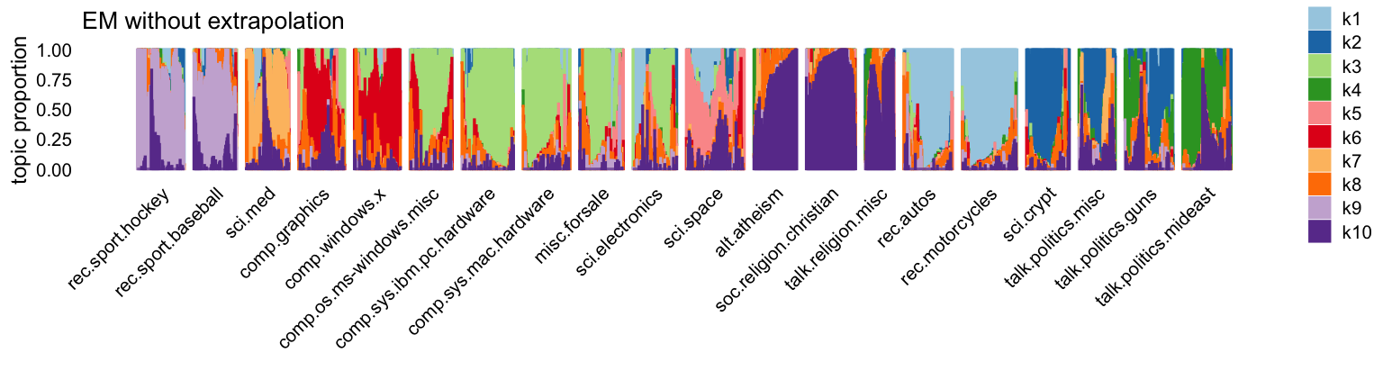
And here are the CD estimates:
L2 <- select_loadings(fit2,rows)$L
p2 <- structure_plot(L2,topics = 1:10,grouping = topics[rows],
                     colors = topic_colors,gap = 10) +
  ggtitle("CD with extrapolation") +
  theme(plot.title = element_text(face = "plain",size = 10))
p2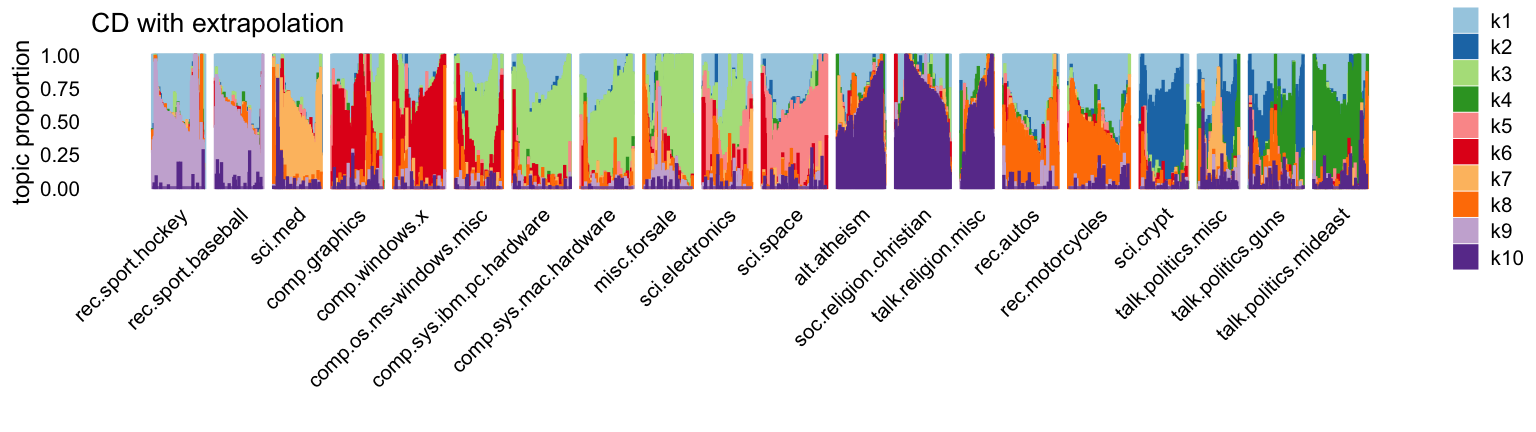
The most striking differences are in topics 1 and 8.
Let’s now extract some “keywords” for a few selected topics by taking words that are at higher frequency in the given topic compared to the other topics. For example, top keywords for topic 9 clearly relate to baseball, hockey and sports more generally:
k <- 9
dat <- data.frame(word = colnames(counts),
                  f0 = apply(fit2$F[,-k],1,max),
                  f1 = fit1$F[,k],
                  f2 = fit2$F[,k])
subset(dat,f0 < 1e-5 & f2 > 1e-3)
#              word           f0           f1          f2
# baseball baseball 1.264878e-18 0.0020675252 0.002855391
# montreal montreal 7.251379e-06 0.0007823897 0.001078615
# bos           bos 1.264878e-18 0.0008482475 0.001169429
# players   players 9.595820e-06 0.0024795989 0.003422507
# hockey     hockey 1.264878e-18 0.0026976069 0.003719034
# det           det 1.264878e-18 0.0008797847 0.001276868
# braves     braves 1.264878e-18 0.0007343485 0.001012404
# playoffs playoffs 1.264878e-18 0.0007673193 0.001057858
# detroit   detroit 1.264878e-18 0.0009964893 0.001392571
# espn         espn 1.264878e-18 0.0008992023 0.001239678
# leafs       leafs 1.264878e-18 0.0007942954 0.001095049
# nhl           nhl 1.264878e-18 0.0012708726 0.001752078
The keywords for topic 1 seem to suggest a “background topic” that captures words that are not specific to any topic:
k <- 1
dat <- data.frame(word = colnames(counts),
                  f0 = apply(fit2$F[,-k],1,max),
                  f1 = fit1$F[,k],
                  f2 = fit2$F[,k])
subset(dat,f0 > 1e-6 & f2/f0 > 5)
#              word           f0           f1           f2
# sure         sure 2.512762e-04 1.090897e-03 1.692536e-03
# just         just 1.076207e-03 4.551963e-03 5.842350e-03
# keeps       keeps 1.817499e-05 6.700066e-05 1.027829e-04
# don           don 6.465096e-04 3.991194e-03 6.548491e-03
# anyway     anyway 1.175301e-04 6.365821e-04 7.084094e-04
# nope         nope 1.028566e-05 3.561286e-05 5.508114e-05
# happens   happens 4.295433e-05 2.128200e-04 3.140891e-04
# wouldn     wouldn 5.921440e-05 5.217093e-04 7.396585e-04
# going       going 1.934898e-04 1.441073e-03 2.156136e-03
# really     really 2.526422e-04 1.844767e-03 2.443492e-03
# shouldn   shouldn 3.461313e-05 1.453972e-04 2.660836e-04
# maybe       maybe 1.235100e-04 8.788490e-04 1.177699e-03
# guess       guess 6.037515e-05 4.870811e-04 7.643763e-04
# worse       worse 3.896588e-05 1.794090e-04 3.210723e-04
# glad         glad 1.560221e-05 9.443811e-05 1.257976e-04
# lot           lot 2.316579e-04 9.727162e-04 1.324099e-03
# complain complain 7.588646e-06 7.343811e-05 8.735658e-05
# aren         aren 9.011923e-05 3.236008e-04 4.946874e-04
# wasting   wasting 9.404078e-06 4.273874e-05 4.860590e-05
# bothered bothered 5.526302e-06 2.487617e-05 5.460924e-05
# fucking   fucking 1.700176e-06 1.568006e-05 3.497150e-05
# stupid     stupid 6.411798e-05 2.708437e-04 3.229429e-04
# scary       scary 5.386777e-06 3.737996e-05 4.461554e-05
# squashed squashed 1.063293e-06 9.245623e-06 6.194854e-06
# sounded   sounded 7.305338e-06 5.979282e-05 3.832783e-05
# hiking     hiking 1.717477e-06 2.150255e-05 9.142511e-06
Finally, topic 8 is a topic that is quite noticeably different between the EM and CD estimates, and indeed based on the keywords, only the CD estimates produce a topic about cars and motorcycles, with keywords such as wheel, riding, bmw, etc:
k <- 8
dat <- data.frame(word = colnames(counts),
                  f0 = apply(fit2$F[,-k],1,max),
                  f1 = fit1$F[,k],
                  f2 = fit2$F[,k])
subset(dat,f0 < 1e-5 & f2 > 5e-4)
#                    word           f0           f1           f2
# wheel             wheel 6.543365e-06 1.683374e-18 0.0009816094
# bmw                 bmw 1.264878e-18 3.192401e-18 0.0015759252
# mustang         mustang 1.264878e-18 1.330000e-18 0.0005921106
# ford               ford 9.643654e-06 1.371222e-04 0.0013342849
# helmet           helmet 9.667809e-06 1.337740e-18 0.0008102502
# di                   di 1.812754e-06 8.805320e-04 0.0007696219
# mov                 mov 1.264878e-18 7.427849e-04 0.0006422123
# cx                   cx 7.585213e-06 6.729076e-04 0.0005761026
# ei                   ei 1.264878e-18 8.218046e-04 0.0007105328
# bike               bike 1.264878e-18 5.693028e-18 0.0038122818
# toyota           toyota 1.264878e-18 1.330000e-18 0.0005875557
# tire               tire 8.870782e-06 1.330000e-18 0.0005369584
# honda             honda 1.264878e-18 3.048671e-18 0.0010657990
# brakes           brakes 1.264878e-18 1.330000e-18 0.0005192353
# brake             brake 5.320512e-06 1.330000e-18 0.0007191107
# tires             tires 4.859009e-06 1.330000e-18 0.0007878724
# callison       callison 1.264878e-18 1.330000e-18 0.0005010166
# bikes             bikes 1.264878e-18 1.483688e-18 0.0008972752
# motorcycles motorcycles 1.264878e-18 1.330000e-18 0.0006285481
# behanna         behanna 1.264878e-18 1.330000e-18 0.0005328995
sessionInfo()
# R version 4.3.3 (2024-02-29)
# Platform: aarch64-apple-darwin20 (64-bit)
# Running under: macOS 15.5
#
# Matrix products: default
# BLAS:   /Library/Frameworks/R.framework/Versions/4.3-arm64/Resources/lib/libRblas.0.dylib
# LAPACK: /Library/Frameworks/R.framework/Versions/4.3-arm64/Resources/lib/libRlapack.dylib;  LAPACK version 3.11.0
#
# locale:
# [1] en_US.UTF-8/en_US.UTF-8/en_US.UTF-8/C/en_US.UTF-8/en_US.UTF-8
#
# time zone: America/Chicago
# tzcode source: internal
#
# attached base packages:
# [1] stats     graphics  grDevices utils     datasets  methods   base
#
# other attached packages:
# [1] cowplot_1.1.3      ggplot2_3.5.0      fastTopics_0.7-25  topicmodels_0.2-16
# [5] Matrix_1.6-5
#
# loaded via a namespace (and not attached):
#  [1] tidyselect_1.2.1    viridisLite_0.4.2   dplyr_1.1.4
#  [4] farver_2.1.1        fastmap_1.1.1       lazyeval_0.2.2
#  [7] promises_1.2.1      digest_0.6.34       lifecycle_1.0.4
# [10] NLP_0.2-1           invgamma_1.1        magrittr_2.0.3
# [13] compiler_4.3.3      rlang_1.1.5         sass_0.4.9
# [16] progress_1.2.3      tools_4.3.3         utf8_1.2.4
# [19] yaml_2.3.8          data.table_1.17.4   knitr_1.45
# [22] prettyunits_1.2.0   labeling_0.4.3      htmlwidgets_1.6.4
# [25] plyr_1.8.9          xml2_1.3.6          Rtsne_0.17
# [28] workflowr_1.7.1     withr_3.0.2         purrr_1.0.2
# [31] grid_4.3.3          stats4_4.3.3        fansi_1.0.6
# [34] git2r_0.33.0        tm_0.7-13           colorspace_2.1-0
# [37] scales_1.3.0        gtools_3.9.5        cli_3.6.4
# [40] rmarkdown_2.26      crayon_1.5.2        ragg_1.2.7
# [43] generics_0.1.3      RcppParallel_5.1.10 httr_1.4.7
# [46] reshape2_1.4.4      pbapply_1.7-2       cachem_1.0.8
# [49] stringr_1.5.1       modeltools_0.2-23   parallel_4.3.3
# [52] vctrs_0.6.5         jsonlite_1.8.8      slam_0.1-50
# [55] hms_1.1.3           mixsqp_0.3-54       ggrepel_0.9.5
# [58] irlba_2.3.5.1       systemfonts_1.0.6   plotly_4.10.4
# [61] jquerylib_0.1.4     tidyr_1.3.1         glue_1.8.0
# [64] uwot_0.2.3          stringi_1.8.3       gtable_0.3.4
# [67] later_1.3.2         quadprog_1.5-8      munsell_0.5.0
# [70] tibble_3.2.1        pillar_1.9.0        htmltools_0.5.8.1
# [73] truncnorm_1.0-9     R6_2.5.1            textshaping_0.3.7
# [76] rprojroot_2.0.4     evaluate_1.0.3      lattice_0.22-5
# [79] highr_0.10          RhpcBLASctl_0.23-42 SQUAREM_2021.1
# [82] ashr_2.2-66         httpuv_1.6.14       bslib_0.6.1
# [85] Rcpp_1.0.12         whisker_0.4.1       xfun_0.42
# [88] fs_1.6.5            pkgconfig_2.0.3