Simulation 2: Real-genotype simulation
Ziang Zhang
2026-09-18
Last updated: 2026-11-04
Checks: 7 0
Knit directory: coderepo-local/
This reproducible R Markdown analysis was created with workflowr (version 1.7.2). The Checks tab describes the reproducibility checks that were applied when the results were created. The Past versions tab lists the development history.
Great! Since the R Markdown file has been committed to the Git repository, you know the exact version of the code that produced these results.
Great job! The global environment was empty. Objects defined in the global environment can affect the analysis in your R Markdown file in unknown ways. For reproduciblity it’s best to always run the code in an empty environment.
The command set.seed(20251109) was run prior to running
the code in the R Markdown file. Setting a seed ensures that any results
that rely on randomness, e.g. subsampling or permutations, are
reproducible.
Great job! Recording the operating system, R version, and package versions is critical for reproducibility.
Nice! There were no cached chunks for this analysis, so you can be confident that you successfully produced the results during this run.
Great job! Using relative paths to the files within your workflowr project makes it easier to run your code on other machines.
Great! You are using Git for version control. Tracking code development and connecting the code version to the results is critical for reproducibility.
The results in this page were generated with repository version fe649c2. See the Past versions tab to see a history of the changes made to the R Markdown and HTML files.
Note that you need to be careful to ensure that all relevant files for
the analysis have been committed to Git prior to generating the results
(you can use wflow_publish or
wflow_git_commit). workflowr only checks the R Markdown
file, but you know if there are other scripts or data files that it
depends on. Below is the status of the Git repository when the results
were generated:
Ignored files:
    Ignored:    .DS_Store
    Ignored:    .Rhistory
    Ignored:    .Rproj.user/
    Ignored:    Rplots.pdf
    Ignored:    analysis/.DS_Store
    Ignored:    analysis/.Rhistory
    Ignored:    code/.DS_Store
    Ignored:    code/.Rhistory
    Ignored:    code/revision_simulations/.DS_Store
    Ignored:    data/appendixB/
    Ignored:    data/dynamic_eQTL_real/
    Ignored:    data/revision_simulations/
    Ignored:    data/toy_example/
    Ignored:    output/dynamic_eQTL_real/
    Ignored:    output/pdf/
    Ignored:    output/playwright/
    Ignored:    output/revision_simulations/
    Ignored:    scripts/

Untracked files:
    Untracked:  code/revision_simulations/internal/per_unit_enhancer_enrichment/
    Untracked:  code/revision_simulations/internal/per_unit_expression_correlation/compare_corshrink_versions.R
    Untracked:  code/revision_simulations/internal/per_unit_expression_correlation/diagnose_discordant_calls.R
    Untracked:  code/revision_simulations/internal/per_unit_expression_correlation/diagnose_smooth_mismatch.R
    Untracked:  code/revision_simulations/internal/per_unit_expression_correlation/extract_perunit_lfdr.R
    Untracked:  code/revision_simulations/internal/per_unit_expression_correlation/plot_call_venns.R
    Untracked:  code/revision_simulations/internal/per_unit_expression_correlation/plot_class_variograms.R
    Untracked:  code/revision_simulations/internal/per_unit_expression_correlation/plot_corshrink_result.R
    Untracked:  code/revision_simulations/internal/per_unit_expression_correlation/plot_corshrink_versions.R
    Untracked:  code/revision_simulations/internal/per_unit_expression_correlation/plot_cs_vs_diagonal.R
    Untracked:  code/revision_simulations/internal/per_unit_expression_correlation/plot_day0_day1_distribution.R
    Untracked:  code/revision_simulations/internal/per_unit_expression_correlation/plot_mechanism_summary.R
    Untracked:  code/revision_simulations/internal/per_unit_expression_correlation/plot_perunit_variogram.R
    Untracked:  code/revision_simulations/internal/per_unit_expression_correlation/plot_strober_concordance.R
    Untracked:  code/revision_simulations/internal/per_unit_expression_correlation/plot_three_models.R
    Untracked:  code/revision_simulations/internal/per_unit_expression_correlation/prepare_reference_sets.R
    Untracked:  code/revision_simulations/internal/per_unit_expression_correlation/prototype_corshrink.R
    Untracked:  code/revision_simulations/internal/per_unit_expression_correlation/recover_design_factor.R
    Untracked:  code/revision_simulations/internal/per_unit_expression_correlation/test_corshrink_reimplementation.R
    Untracked:  code/revision_simulations/internal/posterior_interval_coverage/
    Untracked:  code/revision_simulations/internal/r3_stage1_method_comparison/plot_pi0_before_after.py
Note that any generated files, e.g. HTML, png, CSS, etc., are not included in this status report because it is ok for generated content to have uncommitted changes.
These are the previous versions of the repository in which changes were
made to the R Markdown
(analysis/functional_testing_simulation.rmd) and HTML
(docs/functional_testing_simulation.html) files. If you’ve
configured a remote Git repository (see ?wflow_git_remote),
click on the hyperlinks in the table below to view the files as they
were in that past version.
| File | Version | Author | Date | Message |
|---|---|---|---|---|
| Rmd | fe649c2 | Ziang Zhang | 2026-11-04 | Clean up unlinked internal pages, rename analysis pages, and polish website prose |
| html | fe649c2 | Ziang Zhang | 2026-11-04 | Clean up unlinked internal pages, rename analysis pages, and polish website prose |
Overview
This simulation evaluates dynamic eQTL screening followed by temporal classification. It uses ten Monte Carlo seeds and two truth mechanisms: broad random B-spline trajectories and compact raised-cosine trajectories. The analysis proceeds in two stages:
- Compare BF-adjusted FASH-IWP1, BF-adjusted FASH-linear, and direct
linear and quadratic interaction tests for dynamic discovery across
nominal FDR levels from
0.005through0.20, using all6,362units. - At the fixed threshold \(q_{\mathrm{dyn}}=0.05\), classify the FASH-IWP1 dynamic discoveries as Early, Middle, Late, or Switch, separately for each functional, using \(q_{\mathrm{func}}=0.05\).
For donor \(i\), unit \(j\), and observed time \(t\),
\[ Y_{ijt}=\alpha_{jt}+G_{ij}\beta_j(t)+X_i^T\gamma_{jt}+\epsilon_{ijt}, \qquad \epsilon_{ijt}\sim N(0,1). \]
For each seed, one tested cis variant is sampled uniformly for each
of the 6,362 tested genes, and its YRI dosage vector is
retained for the same 19 donors. Each replicate has
16 time points and five standardized covariates. Per-time
regressions include an intercept, genotype, and five covariates; their
t-adjusted standard errors use 12 residual degrees of freedom. The
dynamic, constant, and zero-effect counts are exactly
1,272/2,545/2,545, with truth classes balanced across
empirical-MAF deciles.
The dynamic effects have Early/Middle/Late probabilities
0.29/0.42/0.29. Switch status is balanced within each
location, giving six exact cell counts
185/184/267/267/185/184. The final trajectory, including
its random genetic main effect, must satisfy the assigned location and
Switch margins. Early is \(t\leq3\),
Middle is \(3<t<12\), and Late is
\(t\geq12\) on the dense 0.1-day grid;
Switch uses threshold 0.25. The two mechanisms retain the same truth
contract:
- Broad effects are cubic B-splines with six independent standard-normal coefficients, centered over the observed times and scaled to maximum absolute deviation 2.
- Compact effects contain one, two, or three raised-cosine peaks with half-width 1.5 and are scaled to centered RMS 0.9.
Examples of true effect curves
Figure 1 shows six examples from seed 12345: broad
B-spline effects classified as Early, Middle, or Late (A-C), and
transient raised-cosine effects with one, two, or three generating peaks
(D-F). Each panel shows the first eligible unit in each category. Black
points are estimated effects, gray bars span \(\pm 2\) reported standard errors, and
orange curves show the true \(\beta_j(t)\), including the genetic main
effect.
# Select one stored example per category.
example_members <- unique(truth_example_pool[, c("truth_mechanism", "target",
  "unit_index", "pair_key", "true_functional", "peak_count")])
example_members <- example_members[order(example_members$unit_index), ]
panel_labels <- c("A. Broad: Early", "B. Broad: Middle", "C. Broad: Late",
                  "D. Transient: one peak", "E. Transient: two peaks",
                  "F. Transient: three peaks")
selected_examples <- do.call(rbind, lapply(seq_along(panel_labels), function(i) {
  eligible <- if (i <= 3L) {
    example_members$truth_mechanism == "random_bspline" &
      example_members$target == c("early", "middle", "late")[[i]] &
      example_members$true_functional > 0
  } else {
    example_members$truth_mechanism == "raised_cosine" &
      !is.na(example_members$peak_count) & example_members$peak_count == i - 3L
  }
  member <- head(example_members[eligible, c("truth_mechanism", "unit_index",
    "pair_key", "peak_count")], 1L)
  stopifnot(nrow(member) == 1L)
  member$panel <- panel_labels[[i]]
  member
}))
# Match stored peak counts to the generating labels.
peak_labels <- readRDS(file.path(project_root,
  "output/revision_simulations/internal/r3_peak_stratified_power_20260918",
  "peak_labels.rds"))$records[["12345"]]$units
transient_examples <- selected_examples[4:6, ]
stopifnot(identical(transient_examples$peak_count, 1:3),
  identical(transient_examples$peak_count,
    peak_labels$peak_count[match(transient_examples$pair_key, peak_labels$pair_key)]))
example_curves <- merge(unique(truth_example_pool[, c("truth_mechanism",
  "unit_index", "pair_key", "time", "true_effect")]), selected_examples,
  by = c("truth_mechanism", "unit_index", "pair_key"), sort = FALSE)
example_observed <- merge(attr(truth_example_pool, "observed"), selected_examples,
  by = c("truth_mechanism", "unit_index", "pair_key"), sort = FALSE)
example_curves$panel <- factor(example_curves$panel, levels = panel_labels)
example_observed$panel <- factor(example_observed$panel, levels = panel_labels)
stopifnot(!anyNA(example_curves$panel), !anyNA(example_observed$panel),
  all(table(example_curves$panel) == 151L),
  all(table(example_observed$panel) == 16L))

# Plot estimated effects with +/-2 SE and orange truth.
ggplot2::ggplot(example_observed, ggplot2::aes(time, estimate)) +
  ggplot2::geom_errorbar(ggplot2::aes(ymin = estimate - 2 * se,
    ymax = estimate + 2 * se), width = 0, color = "grey55", linewidth = 0.35) +
  ggplot2::geom_point(size = 1.15, color = "black") +
  ggplot2::geom_line(data = example_curves, ggplot2::aes(time, true_effect),
    color = "#D55E00", linewidth = 0.8) +
  ggplot2::facet_wrap(~ panel, ncol = 3, scales = "free_y") +
  ggplot2::scale_x_continuous(breaks = c(0, 5, 10, 15)) +
  ggplot2::labs(x = "Time (days)", y = "Effect") +
  ggplot2::theme_bw(base_size = 11) +
  ggplot2::theme(panel.grid.minor = ggplot2::element_blank(),
    strip.text = ggplot2::element_text(size = 10),
    axis.text = ggplot2::element_text(size = 9))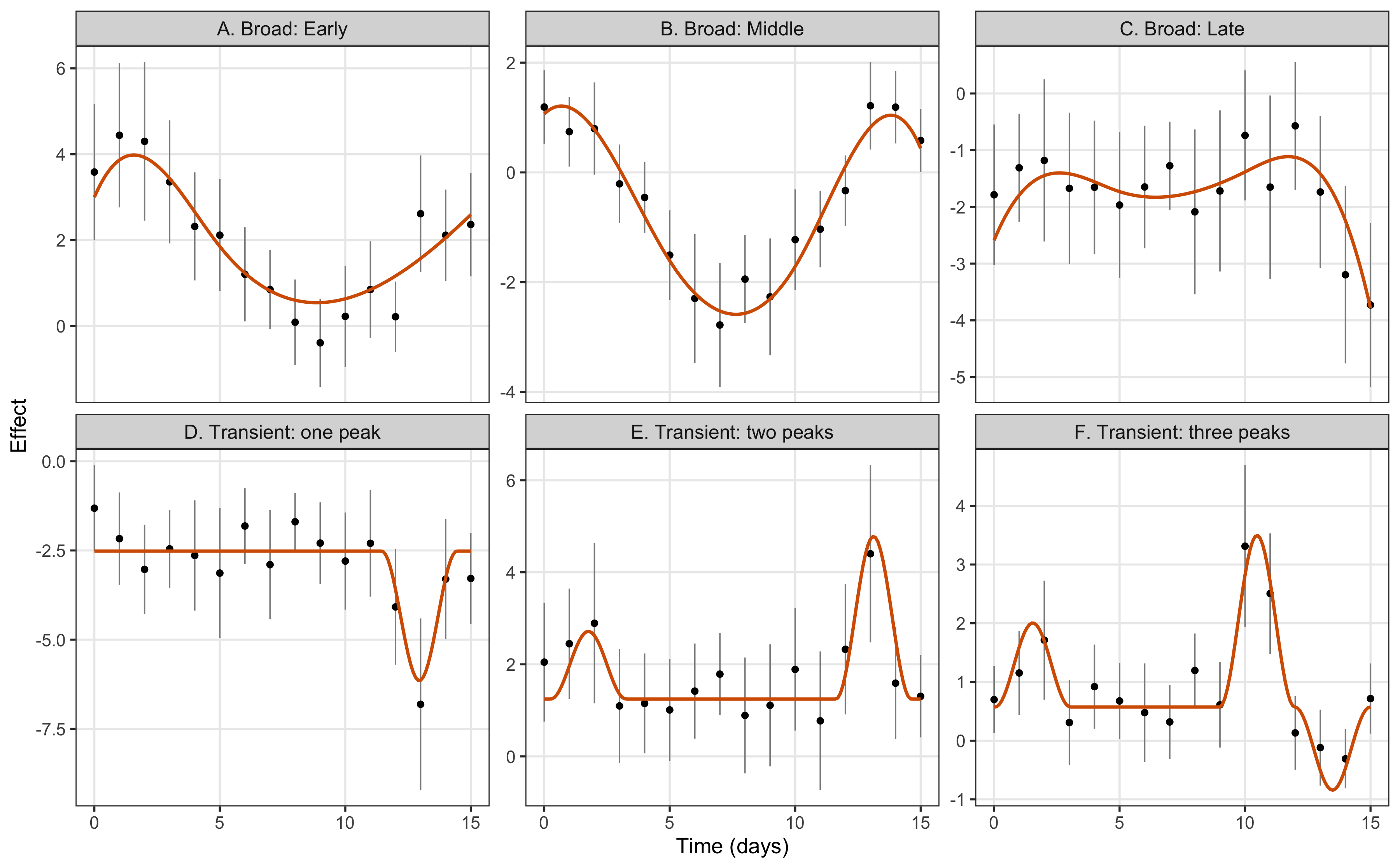
Figure 1. Six representative simulated trajectories. A-C: broad B-spline effects with Early, Middle, and Late truth, respectively. D-F: transient raised-cosine effects with one, two, and three generating peaks, respectively. Each panel shows one unit: black points are estimated effects, gray bars span +/-2 reported standard errors, and the orange curve is the true effect. Panels use separate effect scales.
| Version | Author | Date |
|---|---|---|
| fe649c2 | Ziang Zhang | 2026-11-04 |
Stage 1: dynamic discovery across alpha
FASH-IWP1 and FASH-linear share the unrestricted constant null, the
one-day predictive-SD grid (zero plus 51 positive values from \(\exp(-5)\) to 1), and
penalty = 10. FASH-linear uses a finite mixture of Gaussian
linear slopes. Both fits use the pinned BF update, which retains the
conditional alternative mixture and updates its total weight against the
constant null.
The direct linear LRT tests the genotype-by-time term; the quadratic LRT jointly tests the linear and quadratic interaction terms. Their eFDR uses 100 donor-level permutations, with expression trajectories and covariates permuted together relative to genotype. The direct tests are supplied with the true \(\pi_0=5090/6362\); FASH estimates its null weight. All methods use the same simulated data. FASH receives per-time regression summaries, while the direct tests receive individual-level data.
Let \(D_m(\alpha)\) be the discoveries for method \(m\). FASH uses cumulative mean lfdr, and direct tests use monotone permutation eFDR q-values. For each replicate,
\[ \mathrm{Power}_m(\alpha)=\frac{|D_m(\alpha)\cap H_1|}{|H_1|}, \qquad \mathrm{FDP}_m(\alpha)= \frac{|D_m(\alpha)\cap H_0|}{\max\{|D_m(\alpha)|,1\}}. \]
The curves show the ten-seed means of power and FDP (empirical FDR). Ribbons are pointwise replicate minima and maxima. Each panel is one truth mechanism; the vertical line marks \(\alpha=0.05\), and the FDR diagonal marks nominal calibration.
# FASH: rank all-unit lfdr values and select by their cumulative mean.
lfdr_order <- order(lfdr, unit_index)
fdr <- cumsum(lfdr[lfdr_order]) / seq_along(lfdr_order)
fash_calls <- lfdr_order[fdr <= alpha]

# Direct LRTs: apply the same donor permutations to both interaction degrees.
permutation_null <- compute_direct_interaction_permutation_null(
  out = individual_level_data,
  n_permutations = 100L,
  interaction_degrees = c(1L, 2L),
  seed = seed + 10000L,
  permute_covariates_with_expression = TRUE,
  num_cores = num_cores
)
direct_qvalues <- empirical_fdr_qvalues(
  observed_pvalues = observed_lrt$pvalue,
  null_pvalues = as.vector(permutation_null$null_pvalues[[degree_label]]),
  pi0_method = "fixed",
  fixed_pi0 = 5090 / 6362
)$qvalue
direct_calls <- which(direct_qvalues <= alpha)
Power as a function of alpha
# Select the four main-comparison methods.
power_curves <- stage1_summary[
  stage1_summary$method %in% report$contract$display_methods,
  c("truth_mechanism", "method", "alpha", "mean_power", "power_min", "power_max")
]
power_curves <- power_curves[order(
  power_curves$truth_mechanism,
  match(power_curves$method, report$contract$display_methods),
  power_curves$alpha
), ]
r3c_plot_stage1(power_curves, metric = "power")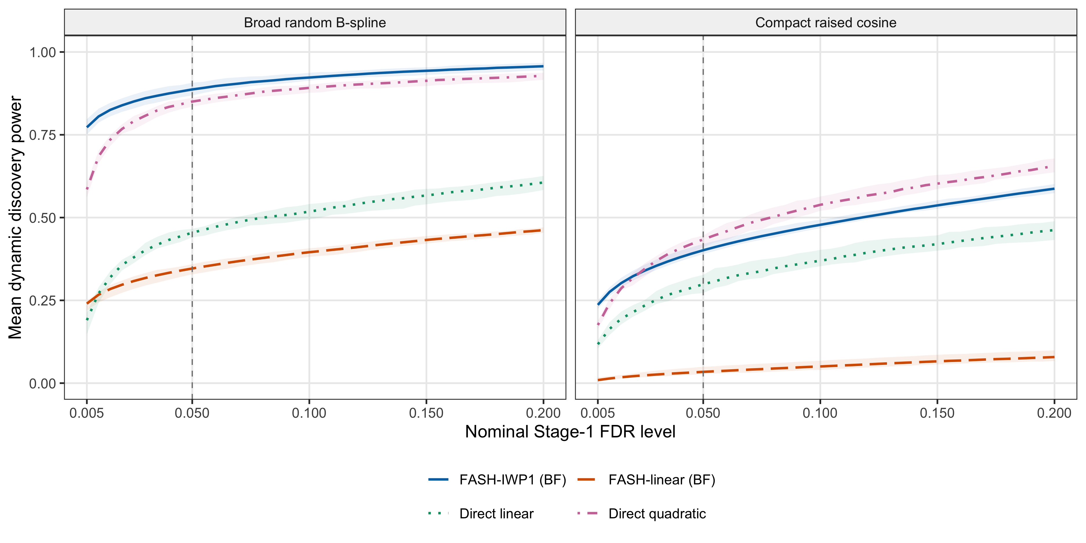
Figure 2. Dynamic discovery power for BF-adjusted FASH-IWP1, BF-adjusted FASH-linear, and direct linear and quadratic interaction tests. Panels show broad random B-spline and compact raised-cosine truth; curves are ten-seed means and ribbons are pointwise replicate minima and maxima. Direct-test eFDR uses the true null proportion and 100 donor permutations.
| Version | Author | Date |
|---|---|---|
| fe649c2 | Ziang Zhang | 2026-11-04 |
Compact-truth power by number of peaks
We split the compact-truth power comparison by the number of generating raised-cosine peaks. For each seed and group, power is the fraction of that group’s true dynamic units selected using the original global method scores and thresholds. The three strata exhaust the dynamic units; curves average these within-group powers across the same ten seeds. Each replicate contains 426, 424, and 422 true dynamic units with one, two, and three peaks, respectively.
# Each stratum's denominator is all true dynamic units with that peak count.
peak_curves <- peak_power$summary[
  peak_power$summary$method %in% report$contract$display_methods,
  c("peak_count", "method", "alpha", "mean_power", "power_min", "power_max")
]
method_labels <- setNames(c("FASH-IWP1 (BF)", "FASH-linear (BF)",
  "Direct linear", "Direct quadratic"), report$contract$display_methods)
peak_curves$method_label <- factor(method_labels[peak_curves$method],
  levels = unname(method_labels))
peak_curves$peak_group <- factor(peak_curves$peak_count, levels = 1:3,
  labels = c("1 peak\n426 units per seed", "2 peaks\n424 units per seed",
             "3 peaks\n422 units per seed"))
stopifnot(nrow(peak_curves) == 480L, !anyNA(peak_curves$method_label),
          !anyNA(peak_curves$peak_group))
method_colors <- setNames(c("#0072B2", "#D55E00", "#009E73", "#CC79A7"),
  unname(method_labels))
method_lines <- setNames(c("solid", "longdash", "dotted", "dotdash"),
  unname(method_labels))
ggplot2::ggplot(peak_curves, ggplot2::aes(alpha, mean_power,
    color = method_label, fill = method_label, linetype = method_label)) +
  ggplot2::geom_ribbon(ggplot2::aes(ymin = power_min, ymax = power_max),
    alpha = 0.09, color = NA, show.legend = FALSE) +
  ggplot2::geom_line(linewidth = 0.8) +
  ggplot2::geom_vline(xintercept = 0.05, color = "grey50",
    linetype = "dashed", linewidth = 0.4) +
  ggplot2::facet_wrap(~peak_group, nrow = 1) +
  ggplot2::scale_color_manual(values = method_colors, drop = FALSE) +
  ggplot2::scale_fill_manual(values = method_colors, drop = FALSE) +
  ggplot2::scale_linetype_manual(values = method_lines, drop = FALSE) +
  ggplot2::scale_x_continuous(breaks = c(0.005, 0.05, 0.10, 0.15, 0.20)) +
  ggplot2::coord_cartesian(ylim = c(0, 1)) +
  ggplot2::labs(x = "Nominal Stage-1 FDR level", y = "Mean within-group dynamic power",
    color = NULL, fill = NULL, linetype = NULL) +
  ggplot2::theme_bw(base_size = 12) +
  ggplot2::theme(legend.position = "bottom", panel.grid.minor = ggplot2::element_blank(),
    strip.background = ggplot2::element_rect(fill = "grey95")) +
  ggplot2::guides(color = ggplot2::guide_legend(nrow = 2, byrow = TRUE))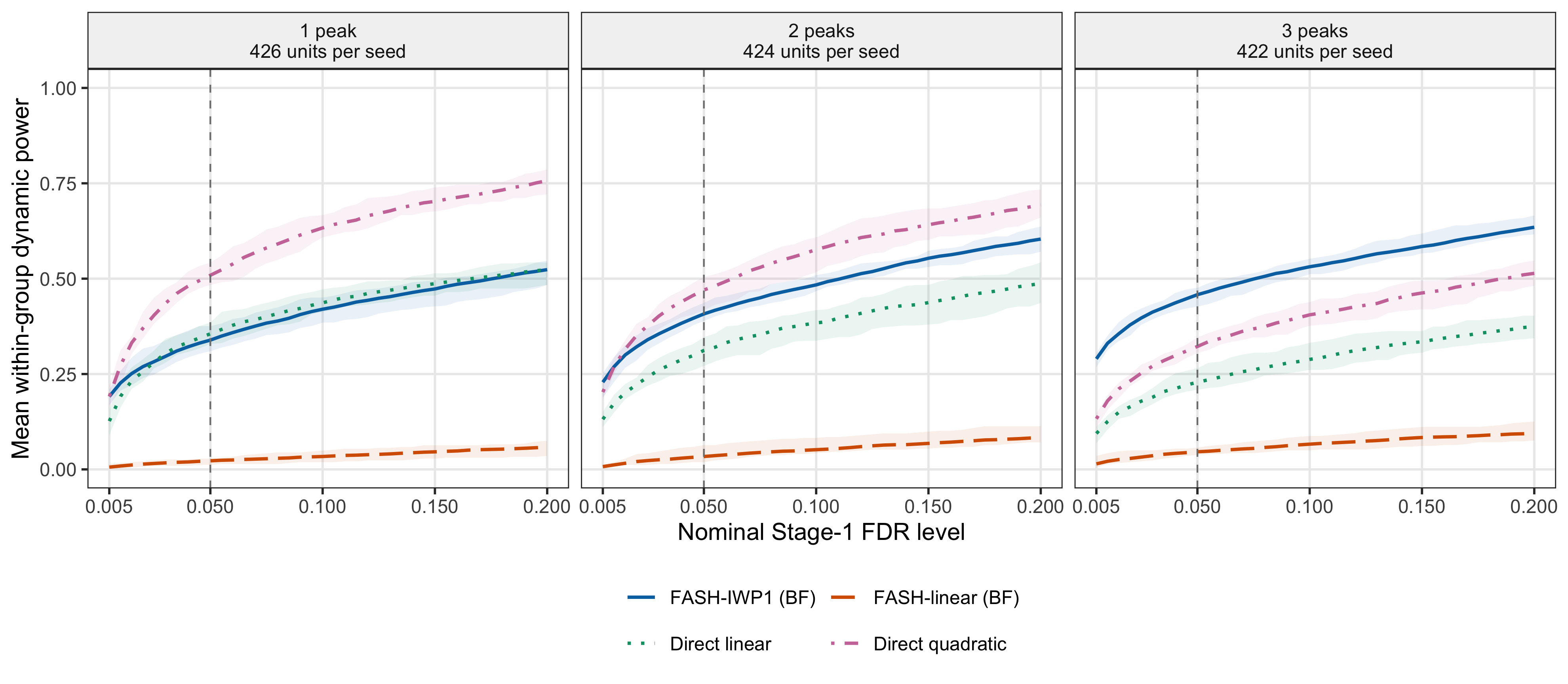
Figure 3. Dynamic discovery power under compact raised-cosine truth, stratified by one, two, or three generating peaks. All four methods retain their original global discovery thresholds. Each curve is the ten-seed mean of within-group power; ribbons show pointwise replicate minima and maxima. The vertical line marks alpha = 0.05.
| Version | Author | Date |
|---|---|---|
| fe649c2 | Ziang Zhang | 2026-11-04 |
At \(\alpha=0.05\), direct quadratic minus BF-adjusted FASH-IWP1 mean power is +17.0, +6.3, and -13.6 percentage points for one, two, and three peaks, respectively. Figure 5 reports the corresponding overall empirical FDR comparison.
Power by temporal category under both truth mechanisms
We split both the broad and compact truth comparisons by true Early, Middle, and Late category, with 369, 534, and 369 dynamic units per seed under each mechanism. Each group includes both Switch and non-Switch units. Power uses all true dynamic units in that category as its denominator and the original global discovery thresholds. This summarizes Stage-1 discovery within true temporal categories; Stage-2 conditional classification is evaluated separately below.
# Each denominator is all true dynamic units with a positive temporal functional.
location_curves <- location_power$summary[
  location_power$summary$method %in% report$contract$display_methods,
  c("truth_mechanism", "target", "method", "alpha", "mean_power", "power_min", "power_max")
]
method_labels <- setNames(c("FASH-IWP1 (BF)", "FASH-linear (BF)",
  "Direct linear", "Direct quadratic"), report$contract$display_methods)
location_curves$method_label <- factor(method_labels[location_curves$method],
  levels = unname(method_labels))
location_curves$location_group <- factor(location_curves$target,
  levels = c("early", "middle", "late"),
  labels = c("Early\n369 units per seed", "Middle\n534 units per seed",
             "Late\n369 units per seed"))
location_curves$mechanism <- factor(location_curves$truth_mechanism,
  levels = c("random_bspline", "raised_cosine"),
  labels = c("Broad random B-spline", "Compact raised cosine"))
stopifnot(nrow(location_curves) == 960L, !anyNA(location_curves$mechanism), !anyNA(location_curves$method_label),
          !anyNA(location_curves$location_group))
method_colors <- setNames(c("#0072B2", "#D55E00", "#009E73", "#CC79A7"),
  unname(method_labels))
method_lines <- setNames(c("solid", "longdash", "dotted", "dotdash"),
  unname(method_labels))
ggplot2::ggplot(location_curves, ggplot2::aes(alpha, mean_power,
    color = method_label, fill = method_label, linetype = method_label)) +
  ggplot2::geom_ribbon(ggplot2::aes(ymin = power_min, ymax = power_max),
    alpha = 0.09, color = NA, show.legend = FALSE) +
  ggplot2::geom_line(linewidth = 0.8) +
  ggplot2::geom_vline(xintercept = 0.05, color = "grey50",
    linetype = "dashed", linewidth = 0.4) +
  ggplot2::facet_grid(mechanism ~ location_group) +
  ggplot2::scale_color_manual(values = method_colors, drop = FALSE) +
  ggplot2::scale_fill_manual(values = method_colors, drop = FALSE) +
  ggplot2::scale_linetype_manual(values = method_lines, drop = FALSE) +
  ggplot2::scale_x_continuous(breaks = c(0.005, 0.05, 0.10, 0.15, 0.20)) +
  ggplot2::coord_cartesian(ylim = c(0, 1)) +
  ggplot2::labs(x = "Nominal Stage-1 FDR level", y = "Mean within-group dynamic power",
    color = NULL, fill = NULL, linetype = NULL) +
  ggplot2::theme_bw(base_size = 12) +
  ggplot2::theme(legend.position = "bottom", panel.grid.minor = ggplot2::element_blank(),
    strip.background = ggplot2::element_rect(fill = "grey95")) +
  ggplot2::guides(color = ggplot2::guide_legend(nrow = 2, byrow = TRUE))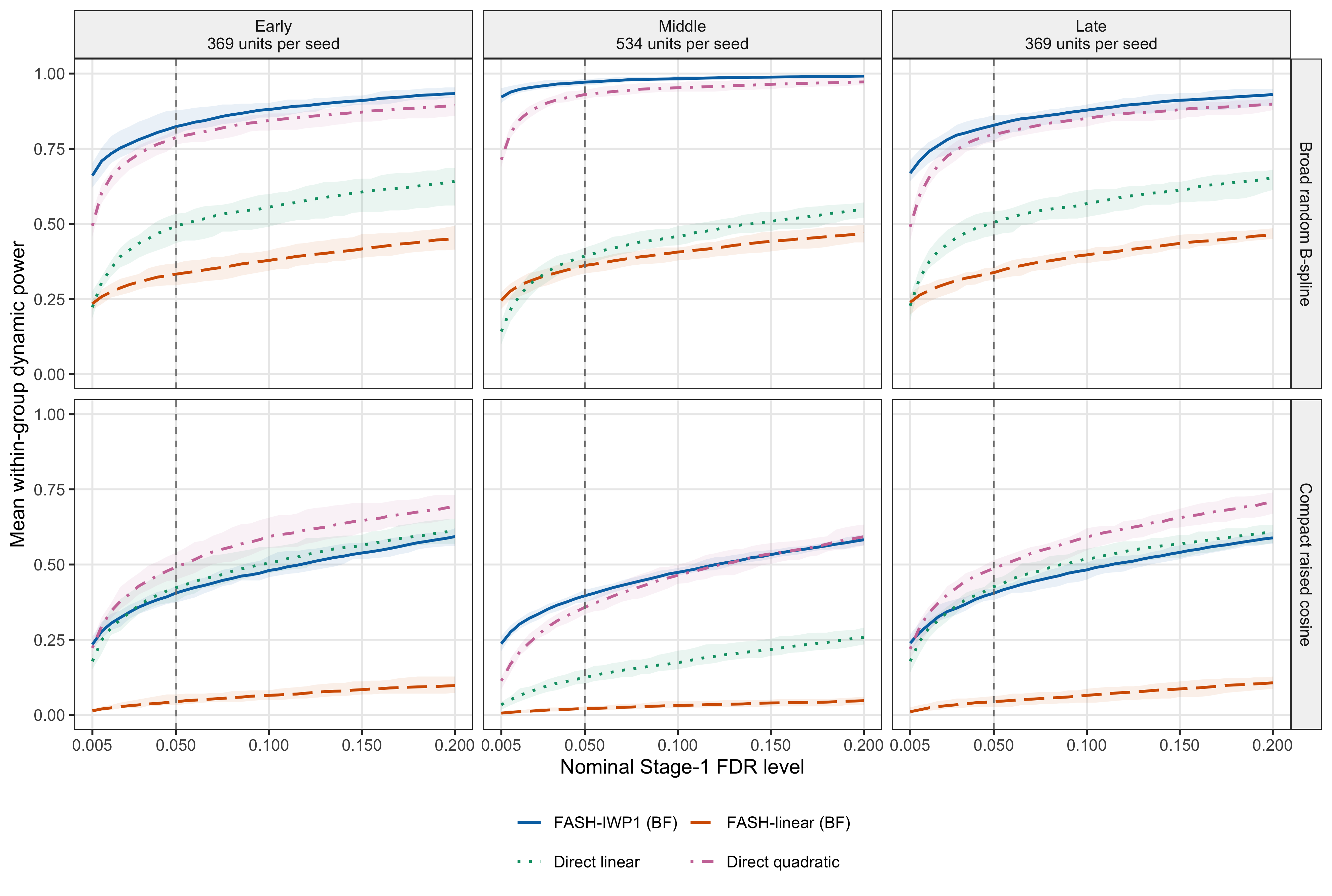
Figure 4. Dynamic discovery power stratified by true Early, Middle, and Late category. Rows show broad random B-spline (top) and compact raised-cosine (bottom) truth. Each stratum includes both Switch and non-Switch units. Curves are ten-seed mean within-category powers using the original global discovery thresholds; ribbons show pointwise replicate minima and maxima. The vertical line marks alpha = 0.05.
| Version | Author | Date |
|---|---|---|
| fe649c2 | Ziang Zhang | 2026-11-04 |
Empirical FDR as a function of alpha
# Use the same truth, method order, and alpha grid as the power comparison.
fdr_curves <- stage1_summary[
  stage1_summary$method %in% report$contract$display_methods,
  c("truth_mechanism", "method", "alpha", "mean_empirical_fdr",
    "empirical_fdr_min", "empirical_fdr_max")
]
fdr_curves <- fdr_curves[order(
  fdr_curves$truth_mechanism,
  match(fdr_curves$method, report$contract$display_methods),
  fdr_curves$alpha
), ]
r3c_plot_stage1(fdr_curves, metric = "fdr")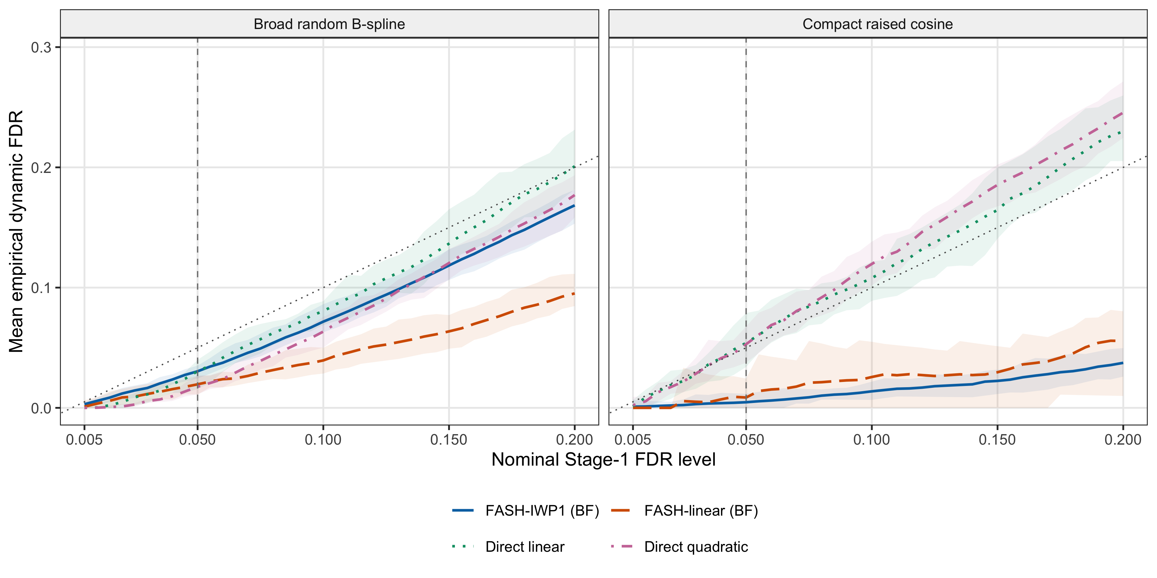
Figure 5. Empirical dynamic FDR for the same four methods and paired datasets. Curves average replicate-specific false-discovery proportions across ten seeds; ribbons are pointwise replicate minima and maxima. The diagonal marks nominal FDR, and the vertical line marks alpha = 0.05.
| Version | Author | Date |
|---|---|---|
| fe649c2 | Ziang Zhang | 2026-11-04 |
At \(\alpha=0.05\), mean power for BF-adjusted FASH-IWP1 and direct quadratic is 0.887 and 0.850 under broad truth, and 0.401 and 0.434 under compact truth. Under compact truth, their mean empirical FDR values are 0.005 and 0.053, respectively; power should therefore be read together with empirical FDR.
Stage 2: conditional functional classification at 0.05
For the remainder of the analysis, \(D(0.05)\) denotes the BF-adjusted FASH-IWP1 discoveries at 0.05. This candidate set remains fixed for Stage 2. The fitted prior remains the full-data prior. For each candidate and each functional, 3,000 posterior draws are evaluated on the dense time grid. The candidate lfsr values are then ranked separately for Early, Middle, Late, and Switch, and calls are made while their cumulative FSR is at most 0.05. The four classifications are evaluated separately and need not be mutually exclusive.
For target \(k\), let \(S_k\subseteq D(0.05)\) be its final calls and let \(T_k\{\beta_j\}>0\) denote true membership. We report
\[ \mathrm{FSR}_k= \frac{\sum_{j\in S_k}\mathbf{1}[T_k\{\beta_j\}\leq0]} {\max(|S_k|,1)}, \]
and conditional classification power
\[ \mathrm{Power}_{k\mid\mathrm{Stage\ 1}}= \frac{\sum_{j\in S_k}\mathbf{1}[T_k\{\beta_j\}>0]} {\sum_{j\in D(0.05)}\mathbf{1}[T_k\{\beta_j\}>0]}. \]
The tables average each replicate-specific rate and call count across the ten seeds.
dynamic_candidates <- r3ts_stage1(
  fdr_table,
  n_units = 6362L,
  q = 0.05
)
lfsr_by_target <- compute_functional_lfsr(
  fit = fit_iwp1_bf,
  functionals = temporal_functionals,
  indices = dynamic_candidates,
  smooth_var = seq(0, 15, by = 0.1),
  num_cores = num_cores,
  seed = functional_posterior_seed
)
stage2_calls <- r3ts_stage2(
  dynamic_candidates,
  lfsr_by_target,
  n_units = 6362L,
  q = 0.05
)
# Select the truth mechanism and retain only the three displayed estimands.
broad_table <- stage2_summary[
stage2_summary$truth_mechanism == "random_bspline",
c("truth_mechanism", "target", "mean_empirical_fsr",
"mean_conditional_classification_power", "mean_calls")
]
broad_table <- broad_table[
match(c("early", "middle", "late", "switch"), broad_table$target),
]
r3ts10_show_table(
r3ts10_format_stage2_table(broad_table, "random_bspline"),
paste(
"Table 1. Ten-seed mean Stage-2 results under broad random B-spline truth.",
"Classification power is conditional on true target members retained by",
"Stage 1 at q = 0.05."
)
)| Metric | Early | Middle | Late | Switch |
|---|---|---|---|---|
| Empirical FSR | 0.001 | 0.037 | 0.009 | 0.034 |
| Conditional classification power | 0.285 | 0.914 | 0.294 | 0.919 |
| Mean number of calls | 86.6 | 492.6 | 90.5 | 575.4 |
# Select the truth mechanism and retain only the three displayed estimands.
compact_table <- stage2_summary[
  stage2_summary$truth_mechanism == "raised_cosine",
  c("truth_mechanism", "target", "mean_empirical_fsr",
    "mean_conditional_classification_power", "mean_calls")
]
compact_table <- compact_table[
  match(c("early", "middle", "late", "switch"), compact_table$target),
]
r3ts10_show_table(
  r3ts10_format_stage2_table(compact_table, "raised_cosine"),
  paste(
    "Table 2. Ten-seed mean Stage-2 results under compact raised-cosine truth.",
    "Classification power is conditional on true target members retained by",
    "Stage 1 at q = 0.05."
  )
)| Metric | Early | Middle | Late | Switch |
|---|---|---|---|---|
| Empirical FSR | 0.013 | 0.037 | 0.005 | 0.034 |
| Conditional classification power | 0.083 | 0.198 | 0.085 | 0.824 |
| Mean number of calls | 12.4 | 43.5 | 12.8 | 332.9 |
Stage-1 screening and Stage-2 classification answer distinct questions. The curves quantify which true dynamic effects reach the candidate set; the tables then quantify functional classification among true target members in that set.
Reproducibility
The simulation scripts are in
code/revision_simulations/internal/r3_two_stage_functional_testing_pilot10/
(two-stage functional classification) and
code/revision_simulations/internal/r3_stage1_method_comparison/
(Stage-1 method comparison), using fashr 0.1.43. To rebuild
this page:
Rscript --vanilla -e \
  'workflowr::wflow_build("analysis/functional_testing_simulation.rmd")'
sessionInfo()R version 4.5.1 (2025-06-13)
Platform: aarch64-apple-darwin20
Running under: macOS Sequoia 15.6.1
Matrix products: default
BLAS: /System/Library/Frameworks/Accelerate.framework/Versions/A/Frameworks/vecLib.framework/Versions/A/libBLAS.dylib
LAPACK: /Library/Frameworks/R.framework/Versions/4.5-arm64/Resources/lib/libRlapack.dylib; LAPACK version 3.12.1
locale:
[1] en_CA/en_CA/en_CA/C/en_CA/en_CA
time zone: America/Chicago
tzcode source: internal
attached base packages:
[1] stats graphics grDevices utils datasets methods base
other attached packages:
[1] workflowr_1.7.2
loaded via a namespace (and not attached):
[1] gtable_0.3.6 jsonlite_2.0.0 dplyr_1.1.4 compiler_4.5.1
[5] promises_1.5.0 tidyselect_1.2.1 Rcpp_1.1.1-1.1 stringr_1.6.0
[9] git2r_0.36.2 dichromat_2.0-0.1 callr_3.7.6 later_1.4.4
[13] jquerylib_0.1.4 scales_1.4.0 yaml_2.3.12 fastmap_1.2.0
[17] ggplot2_4.0.3 R6_2.6.1 labeling_0.4.3 generics_0.1.4
[21] knitr_1.50 tibble_3.3.0 rprojroot_2.1.1 RColorBrewer_1.1-3
[25] bslib_0.9.0 pillar_1.11.1 rlang_1.2.0 cachem_1.1.0
[29] stringi_1.8.9 httpuv_1.6.16 xfun_0.55 S7_0.2.2
[33] getPass_0.2-4 fs_1.6.6 sass_0.4.10 otel_0.2.0
[37] cli_3.6.6 withr_3.0.3 magrittr_2.0.5 ps_1.9.1
[41] grid_4.5.1 digest_0.6.39 processx_3.8.6 rstudioapi_0.17.1
[45] lifecycle_1.0.5 vctrs_0.7.3 evaluate_1.0.5 glue_1.8.1
[49] farver_2.1.2 whisker_0.4.1 rmarkdown_2.30 httr_1.4.7
[53] tools_4.5.1 pkgconfig_2.0.3 htmltools_0.5.9