Dynamic eQTL analysis on iPSC
Ziang Zhang
2025-02-21
Last updated: 2026-01-21
Checks: 7 0
Knit directory: fashr-paper-stephenslab/
This reproducible R Markdown analysis was created with workflowr (version 1.7.2). The Checks tab describes the reproducibility checks that were applied when the results were created. The Past versions tab lists the development history.
Great! Since the R Markdown file has been committed to the Git repository, you know the exact version of the code that produced these results.
Great job! The global environment was empty. Objects defined in the global environment can affect the analysis in your R Markdown file in unknown ways. For reproduciblity it’s best to always run the code in an empty environment.
The command set.seed(20251109) was run prior to running
the code in the R Markdown file. Setting a seed ensures that any results
that rely on randomness, e.g. subsampling or permutations, are
reproducible.
Great job! Recording the operating system, R version, and package versions is critical for reproducibility.
Nice! There were no cached chunks for this analysis, so you can be confident that you successfully produced the results during this run.
Great job! Using relative paths to the files within your workflowr project makes it easier to run your code on other machines.
Great! You are using Git for version control. Tracking code development and connecting the code version to the results is critical for reproducibility.
The results in this page were generated with repository version 0b26571. See the Past versions tab to see a history of the changes made to the R Markdown and HTML files.
Note that you need to be careful to ensure that all relevant files for
the analysis have been committed to Git prior to generating the results
(you can use wflow_publish or
wflow_git_commit). workflowr only checks the R Markdown
file, but you know if there are other scripts or data files that it
depends on. Below is the status of the Git repository when the results
were generated:
Ignored files:
    Ignored:    .DS_Store
    Ignored:    .Rhistory
    Ignored:    .Rproj.user/
    Ignored:    analysis/.DS_Store
    Ignored:    analysis/.Rhistory
    Ignored:    code/.DS_Store
    Ignored:    code/.Rhistory
    Ignored:    data/appendixB/
    Ignored:    data/dynamic_eQTL_real/
    Ignored:    data/toy_example/
    Ignored:    output/dynamic_eQTL_real/

Unstaged changes:
    Modified:   .gitignore
    Modified:   analysis/nonlinear_dynamic_eQTL_real.Rmd
    Modified:   output/toy_example/toy_example_11.pdf
    Modified:   output/toy_example/toy_example_12.pdf
    Modified:   output/toy_example/toy_example_21.pdf
    Modified:   output/toy_example/toy_example_22.pdf
Note that any generated files, e.g. HTML, png, CSS, etc., are not included in this status report because it is ok for generated content to have uncommitted changes.
These are the previous versions of the repository in which changes were
made to the R Markdown (analysis/dynamic_eQTL_real.rmd) and
HTML (docs/dynamic_eQTL_real.html) files. If you’ve
configured a remote Git repository (see ?wflow_git_remote),
click on the hyperlinks in the table below to view the files as they
were in that past version.
| File | Version | Author | Date | Message |
|---|---|---|---|---|
| Rmd | 0b26571 | Ziang Zhang | 2026-01-21 | workflowr::wflow_publish("analysis/dynamic_eQTL_real.rmd") |
| html | ebf8a85 | Ziang Zhang | 2026-01-21 | Build site. |
| Rmd | 709663f | Ziang Zhang | 2026-01-21 | workflowr::wflow_publish("analysis/dynamic_eQTL_real.rmd") |
| Rmd | 4c1c6ec | Ziang Zhang | 2026-01-20 | rerun using 5 pcs |
| html | 4c1c6ec | Ziang Zhang | 2026-01-20 | rerun using 5 pcs |
| html | 885ee18 | Ziang Zhang | 2026-01-19 | update code for non-linear dynamic |
| Rmd | 79ff501 | Ziang Zhang | 2026-01-19 | code refactor |
| html | 79ff501 | Ziang Zhang | 2026-01-19 | code refactor |
| html | 0fc1046 | Ziang Zhang | 2025-12-18 | Build site. |
| Rmd | c0e05d7 | Ziang Zhang | 2025-12-18 | workflowr::wflow_publish("analysis/dynamic_eQTL_real.rmd") |
| html | c75cd5f | Ziang Zhang | 2025-12-18 | Build site. |
| Rmd | 27c4197 | Ziang Zhang | 2025-12-18 | workflowr::wflow_publish("analysis/dynamic_eQTL_real.rmd") |
| html | c3e274e | Ziang Zhang | 2025-12-17 | Build site. |
| Rmd | c636ff9 | Ziang Zhang | 2025-12-17 | workflowr::wflow_publish("analysis/dynamic_eQTL_real.rmd") |
| html | 2010ecb | Ziang Zhang | 2025-12-16 | Build site. |
| Rmd | bd29c15 | Ziang Zhang | 2025-12-16 | workflowr::wflow_publish("analysis/dynamic_eQTL_real.rmd") |
| html | 5be62b6 | Ziang Zhang | 2025-12-12 | Build site. |
| Rmd | bb505cf | Ziang Zhang | 2025-12-12 | workflowr::wflow_publish("analysis/dynamic_eQTL_real.rmd") |
| html | 83145cc | Ziang Zhang | 2025-12-12 | Build site. |
| Rmd | aae2964 | Ziang Zhang | 2025-12-12 | workflowr::wflow_publish("analysis/dynamic_eQTL_real.rmd") |
| html | 36a81a3 | Ziang Zhang | 2025-11-09 | Build site. |
| html | d73f3f1 | Ziang Zhang | 2025-11-09 | Build site. |
| Rmd | 9f55956 | Ziang Zhang | 2025-11-09 | workflowr::wflow_publish("analysis/dynamic_eQTL_real.rmd") |
knitr::opts_chunk$set(fig.width = 8, fig.height = 6, message = FALSE, warning = FALSE)

library(fashr)
library(dplyr)
library(tidyr)
library(stringr)
library(purrr)

# plotting / viz
library(ggplot2)
library(ggrepel)

# paths
result_dir <- file.path(getwd(), "output", "dynamic_eQTL_real")
data_dir   <- file.path(getwd(), "data",   "dynamic_eQTL_real")
code_dir   <- file.path(getwd(), "code",   "dynamic_eQTL_real")

# grids
log_prec  <- seq(0, 10, by = 0.2)
fine_grid <- sort(c(0, exp(-0.5 * log_prec)))

# ----------------------------
# small utilities
# ----------------------------
cache_read <- function(path) if (file.exists(path)) readRDS(path) else NULL
cache_write <- function(x, path) {
  dir.create(dirname(path), showWarnings = FALSE, recursive = TRUE)
  saveRDS(x, path)
  x
}

sample_int <- function(n, size, seed = 1L) {
  set.seed(seed)
  sample.int(n, size = min(size, n))
}

# Parse "ENSG..._rs..." keys once
parse_pair_keys <- function(keys) {
  m <- str_match(keys, "^([^_]+)_(.+)$")
  tibble(key = keys, ens_id = m[,2], rs_id = m[,3])
}

# ----------------------------
# biomaRt mapping with cache
# ----------------------------
get_gene_map <- function(ens_ids, cache_path) {
  ens_ids <- unique(as.character(ens_ids))
  cached <- cache_read(cache_path)
  if (!is.null(cached)) return(cached)

  suppressMessages({
    library(biomaRt)
    mart <- useEnsembl(biomart = "genes", dataset = "hsapiens_gene_ensembl")
  })

  mp <- getBM(
    attributes = c("ensembl_gene_id", "hgnc_symbol"),
    filters    = "ensembl_gene_id",
    values     = ens_ids,
    mart       = mart
  ) %>%
    as_tibble() %>%
    distinct()

  cache_write(mp, cache_path)
}

symbol_of <- function(ens_id, map_tbl) {
  s <- map_tbl$hgnc_symbol[match(ens_id, map_tbl$ensembl_gene_id)]
  ifelse(is.na(s) | s == "", ens_id, s)
}

# (optional) symbol -> ensembl (small list); cache too
symbol_to_ens <- function(symbols, cache_path) {
  symbols <- unique(as.character(symbols))
  cached <- cache_read(cache_path)
  if (!is.null(cached)) return(cached)

  suppressMessages({
    library(biomaRt)
    mart <- useEnsembl(biomart = "genes", dataset = "hsapiens_gene_ensembl")
  })

  mp <- getBM(
    attributes = c("hgnc_symbol", "ensembl_gene_id"),
    filters    = "hgnc_symbol",
    values     = symbols,
    mart       = mart
  ) %>% as_tibble() %>% distinct()

  cache_write(mp, cache_path)
}

# ----------------------------
# index selection helpers
# ----------------------------
pick_best_idx_by_gene <- function(ens_id, pair_tbl, lfdr_vec, which = c("min", "max")) {
  which <- match.arg(which)
  cand <- pair_tbl %>% filter(ens_id == !!ens_id) %>% pull(idx)
  if (length(cand) == 0) return(NA_integer_)
  if (which == "min") cand[which.min(lfdr_vec[cand])] else cand[which.max(lfdr_vec[cand])]
}

pick_idxs_for_genes <- function(ens_ids, pair_tbl, lfdr_vec, which = "min") {
  purrr::map_int(ens_ids, ~pick_best_idx_by_gene(.x, pair_tbl, lfdr_vec, which = which))
}

# ----------------------------
# unified plotting
# ----------------------------
fmt_sci <- function(x, digits = 2) {
  if (length(x) == 0L || is.null(x) || is.na(x)) return("NA")
  formatC(as.numeric(x), format = "e", digits = digits)
}

plot_pair_base <- function(idx,
                           datasets,
                           fash_raw,
                           fash_adj,
                           gene_map,
                           p_lin = NULL,
                           p_non = NULL,
                           smooth_var = seq(0, 15, by = 0.1),
                           add_lm = TRUE,
                           add_quad = TRUE,
                           main_prefix = NULL,
                           ylim_type = c("data_fitted", "fitted"),
                           include_zero_line = FALSE) {

  dat <- datasets[[idx]]
  x <- dat$x; y <- dat$y; se <- dat$SE
  w <- 1 / (se^2)

  fitted <- predict(fash_adj, index = idx, smooth_var = smooth_var)

  # if ylim_type is data_fitted, take the max and min:
  ylim_type <- match.arg(ylim_type)
  if (ylim_type == "data_fitted") {
    y_min <- min(y - 2 * se, fitted$lower, na.rm = TRUE)
    y_max <- max(y + 2 * se, fitted$upper, na.rm = TRUE)
  }
  else{
    y_min <- min(fitted$lower, na.rm = TRUE)
    y_max <- max(fitted$upper, na.rm = TRUE)
    range <- y_max - y_min
    y_min <- y_min - 0.2 * range
    y_max <- y_max + 0.2 * y_max
  }

  # titles
  key_parts <- strsplit(names(datasets)[idx], "_", fixed = TRUE)[[1]]
  ens_id <- key_parts[1]
  rs_id  <- key_parts[2]
  key   <- names(datasets)[idx]
  gsym   <- symbol_of(ens_id, gene_map)

  main_txt <- paste0(gsym, ": ", rs_id)
  if (!is.null(main_prefix)) main_txt <- paste0(main_prefix, " ", main_txt)

  # fits
  lin_fit  <- if (add_lm)   lm(y ~ x, weights = w) else NULL
  quad_fit <- if (add_quad) lm(y ~ poly(x, 2, raw = TRUE), weights = w) else NULL
  x_grid   <- if (add_quad) seq(min(x), max(x), length.out = 200) else NULL
  quad_pred <- if (add_quad) predict(quad_fit, newdata = data.frame(x = x_grid)) else NULL

  plot(x, y, pch = 20, col = "black", xlab = "Time", ylab = "Effect Est", ylim = c(y_min, y_max))
  title(main = main_txt)

  arrows(x0 = x, y0 = y - 2 * se, x1 = x, y1 = y + 2 * se,
         length = 0.05, angle = 90, code = 3, col = "black")

  polygon(c(fitted$x, rev(fitted$x)), c(fitted$lower, rev(fitted$upper)),
          col = rgb(1, 0, 0, 0.1), border = NA)
  lines(fitted$x, fitted$mean, col = "red", lwd = 2)

  if (add_lm)   abline(lin_fit, col = "green", lty = 2, lwd = 1)
  if (add_quad) lines(x_grid, quad_pred, col = "purple", lty = 2, lwd = 1)
  if (include_zero_line) abline(h = 0, col = "blue", lty = 2, lwd = 1)

  lfdr_before <- fash_raw$lfdr[idx]
  lfdr_after  <- fash_adj$lfdr[idx]
  p_lin_val <- if (!is.null(p_lin) && !is.null(names(p_lin)) && key %in% names(p_lin)) unname(p_lin[[key]]) else NA_real_

  p_non_val <- if (!is.null(p_non) && !is.null(names(p_non)) && key %in% names(p_non)) unname(p_non[[key]]) else NA_real_

  if (!is.na(p_lin_val) || !is.na(p_non_val)) {

    cap <- sprintf("lfdr = %s (%s), p-value = %s (%s)",
                  fmt_sci(lfdr_after), fmt_sci(lfdr_before),
                  fmt_sci(p_lin_val), fmt_sci(p_non_val))

  } else {

    cap <- sprintf("lfdr (raw) = %s, lfdr (adj) = %s", fmt_sci(lfdr_before), fmt_sci(lfdr_after))

  }

  title(sub = cap, cex.sub = 0.8)
  invisible(NULL)
}

plot_many_pairs <- function(idxs, nrow = 2, ncol = 2, ...) {
  dots <- list(...)
  datasets <- dots$datasets

  idxs <- as.integer(idxs)
  idxs <- idxs[!is.na(idxs)]
  idxs <- idxs[idxs >= 1]
  if (!is.null(datasets)) idxs <- idxs[idxs <= length(datasets)]

  if (length(idxs) == 0L) {
    message("plot_many_pairs: no valid indices to plot.")
    return(invisible(NULL))
  }

  oldpar <- par(no.readonly = TRUE)
  on.exit(par(oldpar), add = TRUE)
  par(mfrow = c(nrow, ncol))

  for (idx in idxs) {
    try(plot_pair_base(idx = idx, ...), silent = TRUE)
  }

  invisible(NULL)
}

# ----------------------------
# Strober loading helpers
# ----------------------------
read_strober <- function(path) {
  read.delim(path) %>%
    as_tibble() %>%
    mutate(key = paste0(ensamble_id, "_", rs_id))
}

# ----------------------------
# lfdr vs p-value scatter helper
# ----------------------------
plot_lfdr_vs_p <- function(fash_tbl, strober_df, pval_cutoff, lfdr_cutoff,
                           gene_map, title_text = "",
                           manual_symbol = NULL) {
  eps <- .Machine$double.eps
  if (is.null(manual_symbol)) manual_symbol <- c()

  df <- fash_tbl %>%
    inner_join(strober_df %>% dplyr::select(key, ensamble_id, pvalue), by = "key") %>%
    mutate(ensamble_id = dplyr::coalesce(ensamble_id, ens_id))

  # min per gene
  df_p <- df %>% dplyr::group_by(ensamble_id) %>% dplyr::slice_min(pvalue, n = 1, with_ties = FALSE) %>% dplyr::ungroup()
  df_l <- df %>% dplyr::group_by(ensamble_id) %>% dplyr::slice_min(lfdr_adj, n = 1, with_ties = FALSE) %>% dplyr::ungroup()

  g <- df_p %>% dplyr::select(ensamble_id, pvalue) %>%
    inner_join(df_l %>% dplyr::select(ensamble_id, lfdr_adj), by = "ensamble_id") %>%
    mutate(
      gene_symbol = symbol_of(ensamble_id, gene_map),
      gene_label  = dplyr::coalesce(unname(manual_symbol[ensamble_id]), gene_symbol, ensamble_id),
      neglog_p    = -log10(pmin(pmax(pvalue, eps), 1)),
      neglog_lfdr = -log10(pmin(pmax(lfdr_adj, eps), 1)),
      category = dplyr::case_when(
        pvalue <= pval_cutoff & lfdr_adj <= lfdr_cutoff ~ "Both",
        pvalue <= pval_cutoff & lfdr_adj >  lfdr_cutoff ~ "Strober only",
        pvalue >  pval_cutoff & lfdr_adj <= lfdr_cutoff ~ "FASH only",
        TRUE ~ "Neither"
      ),
      category = factor(category, levels = c("Both", "FASH only", "Strober only", "Neither"))
    )

  top_strober_only <- g %>% dplyr::filter(category == "Strober only") %>% dplyr::arrange(pvalue) %>% dplyr::slice_head(n = 10)
  top_fash_only    <- g %>% dplyr::filter(category == "FASH only")    %>% dplyr::arrange(lfdr_adj) %>% dplyr::slice_head(n = 10)
  top_both         <- g %>% dplyr::filter(category == "Both")         %>% dplyr::arrange(pvalue + lfdr_adj) %>% dplyr::slice_head(n = 10)
  label_df <- dplyr::bind_rows(top_strober_only, top_fash_only, top_both)

  col_map <- c("Both"="#7B3294","FASH only"="#1B9E77","Strober only"="#D95F02","Neither"="grey80")

  ggplot(g, aes(x = neglog_p, y = neglog_lfdr)) +
    geom_point(data = subset(g, category == "Neither"), color = col_map["Neither"], alpha = 0.25, size = 1.8) +
    geom_point(data = subset(g, category != "Neither"), aes(color = category), alpha = 0.8, size = 2.2) +
    scale_color_manual(values = col_map) +
    geom_vline(xintercept = -log10(pval_cutoff), linetype = "dashed") +
    geom_hline(yintercept = -log10(lfdr_cutoff), linetype = "dashed") +
    geom_text_repel(
      data = label_df, aes(label = gene_label, color = category),
      size = 3, box.padding = 0.3, point.padding = 0.5, max.overlaps = Inf, show.legend = FALSE
    ) +
    theme_minimal() +
    theme(text = element_text(size = 16), axis.text = element_text(size = 14), legend.position = "bottom") +
    labs(title = title_text, x = "-log10(p-value)", y = "-log10(lfdr)", color = NULL)
}
Obtain the effect size of eQTLs
We use the processed (expression & genotype) data of Strober et.al, 2019 to perform the eQTL analysis.
For the association testing, we use a linear regression model for each gene-variant pair at each time point. Following the practice in Strober et.al, we adjust for the first 5 PCs.
The code to perform this step can be found in the script
dynamic_eQTL_real/00_eQTLs.R from the code directory.
After this step, we have the effect size of eQTLs for each gene-variant pair at each time point, as well as its standard error.
Fitting FASH
To fit the FASH model on \(\{\beta_i(t_j), s_{ij}\}_{i\in N,j \in [16]}\), we consider fitting two FASH models:
A FASH model based on first order IWP (testing for dynamic eQTLs: \(H_0: \beta_i(t)=c\)).
A FASH model based on second order IWP (testing for nonlinear-dynamic eQTLs: \(H_0: \beta_i(t)=c_1+c_2t\)).
The code to perform this step can be found in the script
dynamic_eQTL_real/01_fash.R from the code directory.
We will directly load the fitted FASH models from the output directory.
load(file.path(result_dir, "fash_fit1_all.RData"))We will load the datasets from the fitted FASH object:
datasets <- fash_fit1$fash_data$data_list
S_list   <- fash_fit1$fash_data$S
for (i in seq_along(datasets)) datasets[[i]]$SE <- S_list[[i]]

pair_tbl <- parse_pair_keys(names(datasets)) %>%
  mutate(idx = row_number())

all_genes <- unique(pair_tbl$ens_id)

gene_map <- get_gene_map(
  ens_ids = all_genes,
  cache_path = file.path(result_dir, "cache_gene_map.rds")
)
In this analysis, we will focus on the FASH(1) model that assumes a first order IWP and tests for dynamic eQTLs.
Let’s take a quick overview of the fitted FASH model:
log_prec <- seq(0,10, by = 0.2)
fine_grid <- sort(c(0, exp(-0.5*log_prec)))

fash_fit1 <- fash(Y = "beta", smooth_var = "time", S = "SE", data_list = datasets,
                  num_basis = 20, order = 1, betaprec = 0,
                  pred_step = 1, penalty = 10, grid = fine_grid,
                  num_cores = num_cores, verbose = TRUE)
save(fash_fit1, file = "./results/fash_fit1_all.RData")fash_fit1Fitted fash Object
-------------------
Number of datasets: 1009173
Likelihood: gaussian
Number of PSD grid values: 52 (initial), 9 (non-trivial)
Order of Integrated Wiener Process (IWP): 1As well as the estimated priors:
fash_fit1$prior_weights psd prior_weight
1 0.000000000 0.428990301
2 0.006737947 0.114737367
3 0.040762204 0.101515369
4 0.055023220 0.158922393
5 0.100258844 0.029418944
6 0.122456428 0.111020074
7 0.223130160 0.025050394
8 0.367879441 0.022618462
9 1.000000000 0.007726694Problem with \(\pi_0\) estimation
If we measure the significance using the false discovery rate, then it is sensitive to the value of \(\pi_0\). The estimated \(\pi_0\) is 0.4289903, which is way too small to be realistic.
One likely reason could be due to model-misspecification under the alternative hypothesis. To account for this, we will consider the following approaches:
(i): Computing a conservative estimate of \(\pi_0\) based on the BF procedure:
fash_fit1_update <- BF_update(fash_fit1, plot = FALSE)
fash_fit1_update$prior_weights
save(fash_fit1_update, file = paste0(result_dir, "/fash_fit1_update.RData"))
The conservative estimate is 0.9381533, which is much more realistic.
(ii): Instead of looking at the FDR which is based on the estimated \(\pi_0\), we can use the minimum local false sign rate (\(\text{min-lfsr}_i\)) to measure significance: \[ \text{min-lfsr}_i = \min_{t} \left\{ \text{lfsr}(W_i(t)) \right\}, \] where \(W_i(t) = \beta_i(t) - \beta_i(0)\).
Let’s compute the significance using the minimum local false sign rate (\(\text{min-lfsr}_i\)):
smooth_var_refined = seq(0,15, by = 0.1)
min_lfsr_summary1 <- min_lfsr_summary(fash_fit1, num_cores = num_cores, smooth_var = smooth_var_refined)
save(min_lfsr_summary1, file = "./results/min_lfsr_summary1.RData")
min_lfsr_summary1_update <- min_lfsr_summary(fash_fit1_update, num_cores = num_cores, smooth_var = smooth_var_refined)
save(min_lfsr_summary1_update, file = "./results/min_lfsr_summary1_update.RData")
Let’s visualize how the min-lfsr compares with the local false discovery rate (lfdr):
load(file.path(result_dir, "min_lfsr_summary1.RData"))

# sample some indices for easy visualization
sample_indices <- sample_int(length(min_lfsr_summary1$min_lfsr), size = 1e5, seed = 1)

min_lfsr1_unadj <- min_lfsr_summary1$min_lfsr[sample_indices]
lfdr1_vec_unadj <- fash_fit1$lfdr[min_lfsr_summary1$index][sample_indices]

plot(lfdr1_vec_unadj, min_lfsr1_unadj,
     pch = 20, cex = 0.1,
     ylim = c(0,1), xlim = c(0,1),
     xlab = "lfdr", ylab = "min-lfsr", main = "lfdr vs min-lfsr (Un-adjusted)")
lines(c(0,1), c(0,1), col = "red")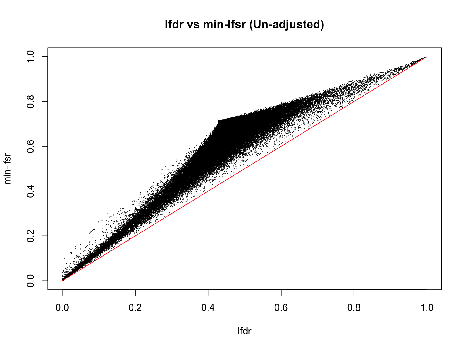
Let’s also visualize the min-lfsr and the lfdr from the BF-updated model:
load(file.path(result_dir, "min_lfsr_summary1_update.RData"))

min_lfsr1 <- min_lfsr_summary1_update$min_lfsr[sample_indices]
lfdr1_vec <- fash_fit1_update$lfdr[min_lfsr_summary1_update$index][sample_indices]

plot(lfdr1_vec, min_lfsr1,
     pch = 20, cex = 0.1,
     ylim = c(0,1), xlim = c(0,1),
     xlab = "lfdr", ylab = "min-lfsr", main = "lfdr vs min-lfsr (BF-adjusted)")
lines(c(0,1), c(0,1), col = "red")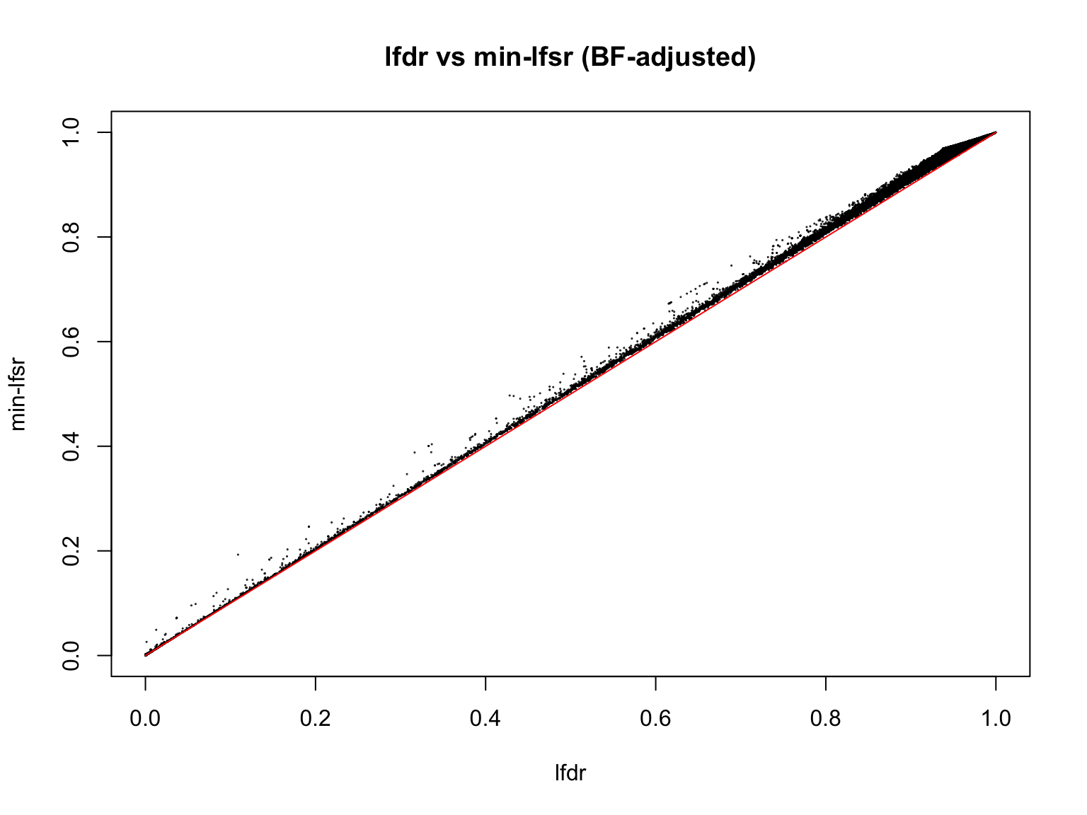
Indeed, the min-lfsr tends to be more conservative than the lfdr, especially when \(\hat{\pi_0}\) has not been adjusted using the BF procedure.
Let’s also assess how does the BF-update of \(\pi_0\) affect the min-lfsr.
plot(min_lfsr1_unadj, min_lfsr1,
     pch = 20, cex = 0.1,
     ylim = c(0,1), xlim = c(0,1),
     xlab = "min-lfsr (unadjusted)", ylab = "min-lfsr", main = "Effect of BF adjustment on min-lfsr")
lines(c(0,1), c(0,1), col = "red")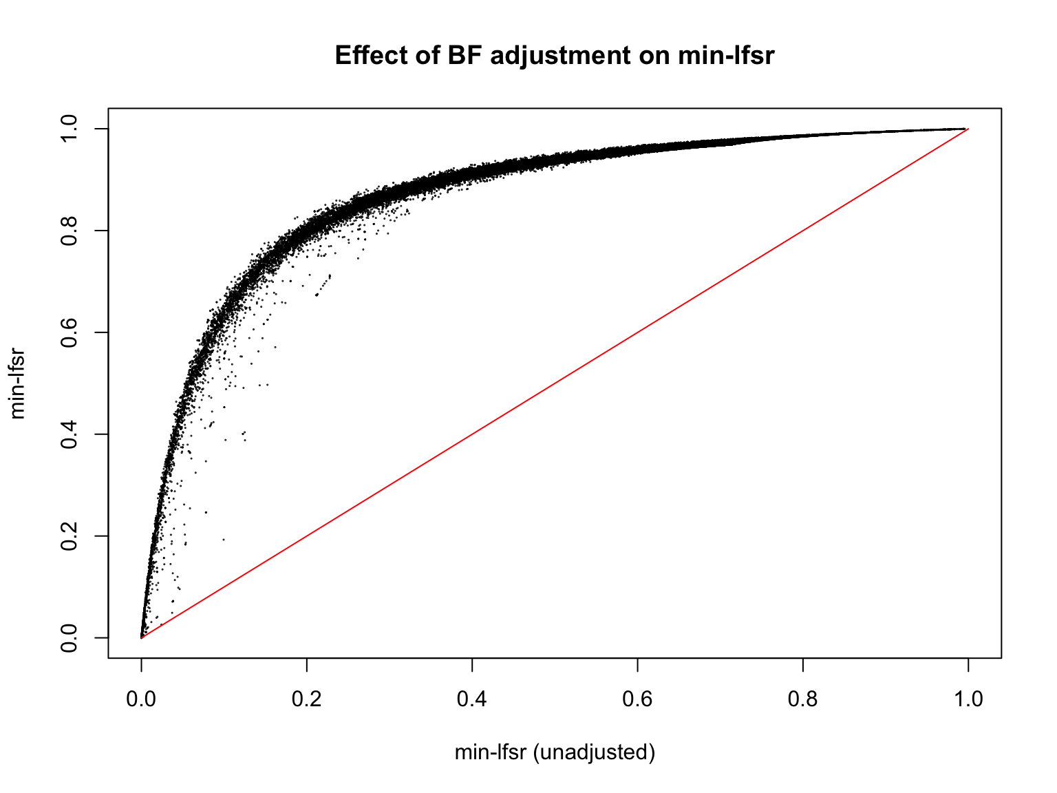
Detecting dynamic eQTLs
We will use the updated FASH model (1) to detect dynamic eQTLs.
alpha <- 0.05

test1 <- fdr_control(fash_fit1_update, alpha = alpha, plot = FALSE)
9205 datasets are significant at alpha level 0.05. Total datasets tested: 1009173. fash_highlighted1 <- test1$fdr_results$index[test1$fdr_results$FDR <= alpha]
test1_before <- fdr_control(fash_fit1, alpha = alpha, plot = FALSE)43860 datasets are significant at alpha level 0.05. Total datasets tested: 1009173. fash_highlighted1_before <- test1_before$fdr_results$index[test1_before$fdr_results$FDR <= alpha]How many pairs are detected as dynamic eQTLs?
pairs_highlighted1 <- names(datasets)[fash_highlighted1]
length(pairs_highlighted1)
[1] 9205length(pairs_highlighted1)/length(datasets)[1] 0.00912133What is the number before the BF adjustment?
pairs_highlighted1_before <- names(datasets)[fash_highlighted1_before]
length(pairs_highlighted1_before)
[1] 43860length(pairs_highlighted1_before)/length(datasets)[1] 0.04346133How many unique genes are detected?
genes_highlighted1 <- unique(
  str_split(test1$significant_units, "_") %>%
  map_chr(1))
length(genes_highlighted1)
[1] 1177length(genes_highlighted1)/length(all_genes)[1] 0.1850047Before the BF adjustment?
genes_highlighted1_before <- unique(pair_tbl$ens_id[pair_tbl$idx %in% fash_highlighted1_before])
length(genes_highlighted1_before)
[1] 3258length(genes_highlighted1_before)/length(all_genes)[1] 0.5121031Let’s see how many pairs and genes remain significant after controlling the min-lfsr:
fash_highlighted1_lfsr <- min_lfsr_summary1_update$index[min_lfsr_summary1_update$fsr <= alpha]
pairs_highlighted1_lfsr <- names(datasets)[fash_highlighted1_lfsr]
length(pairs_highlighted1_lfsr)
[1] 9001length(pairs_highlighted1_lfsr)/length(datasets)[1] 0.008919184genes_highlighted1_lfsr <- unique(pair_tbl$ens_id[pair_tbl$idx %in% fash_highlighted1_lfsr])
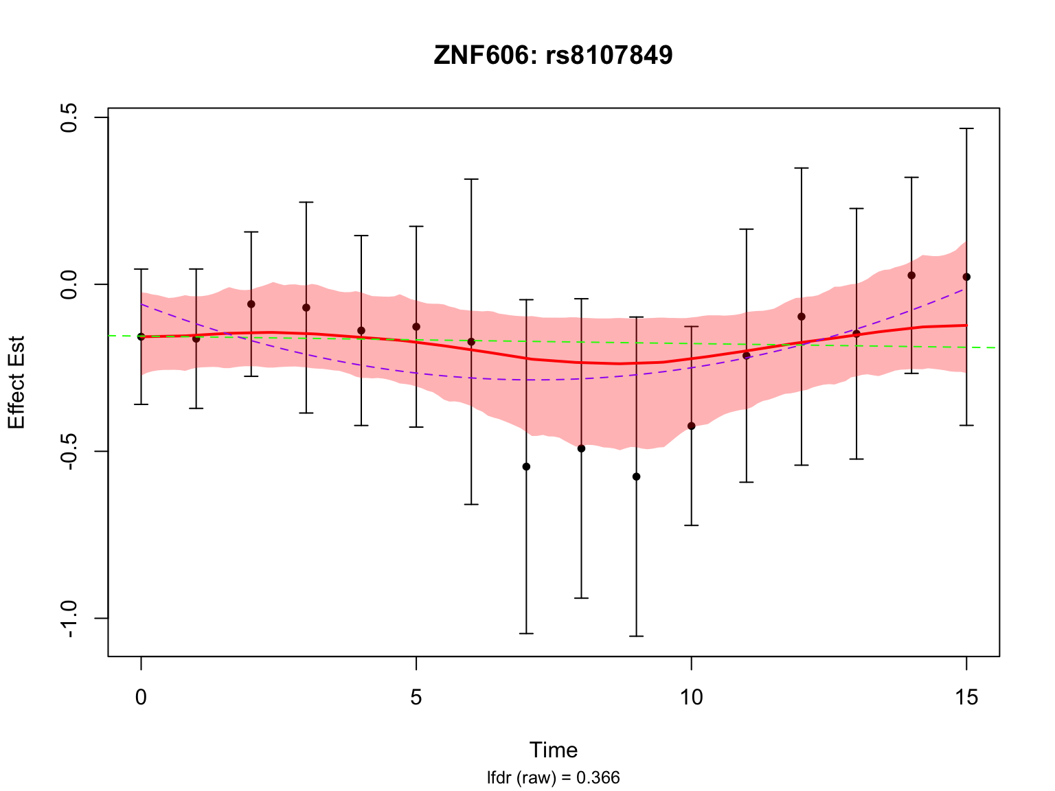
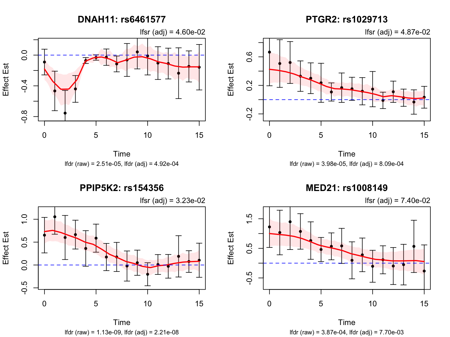
length(genes_highlighted1_lfsr)[1] 1155length(genes_highlighted1_lfsr)/length(all_genes)[1] 0.1815467It seems like once \(\hat{\pi_0}\) is adjusted, there is not much difference between measuring significance using the min-lfsr or the lfdr. From now on, we will consider the pairs that are significant using the lfdr.
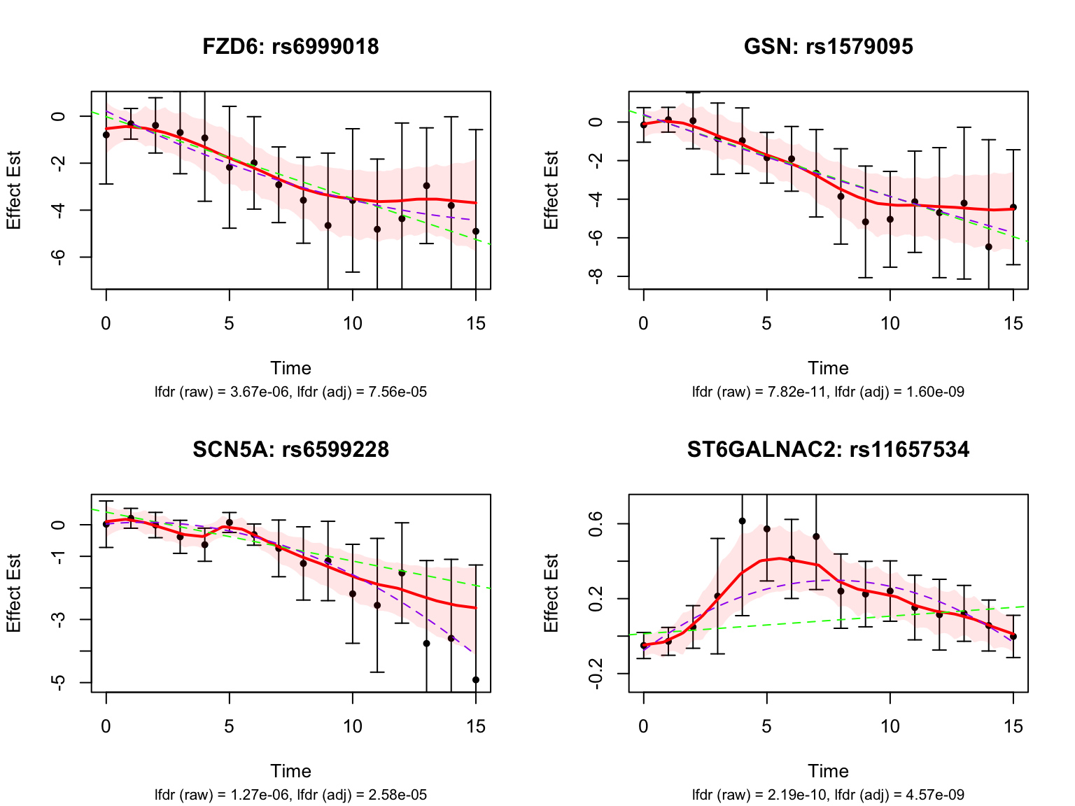
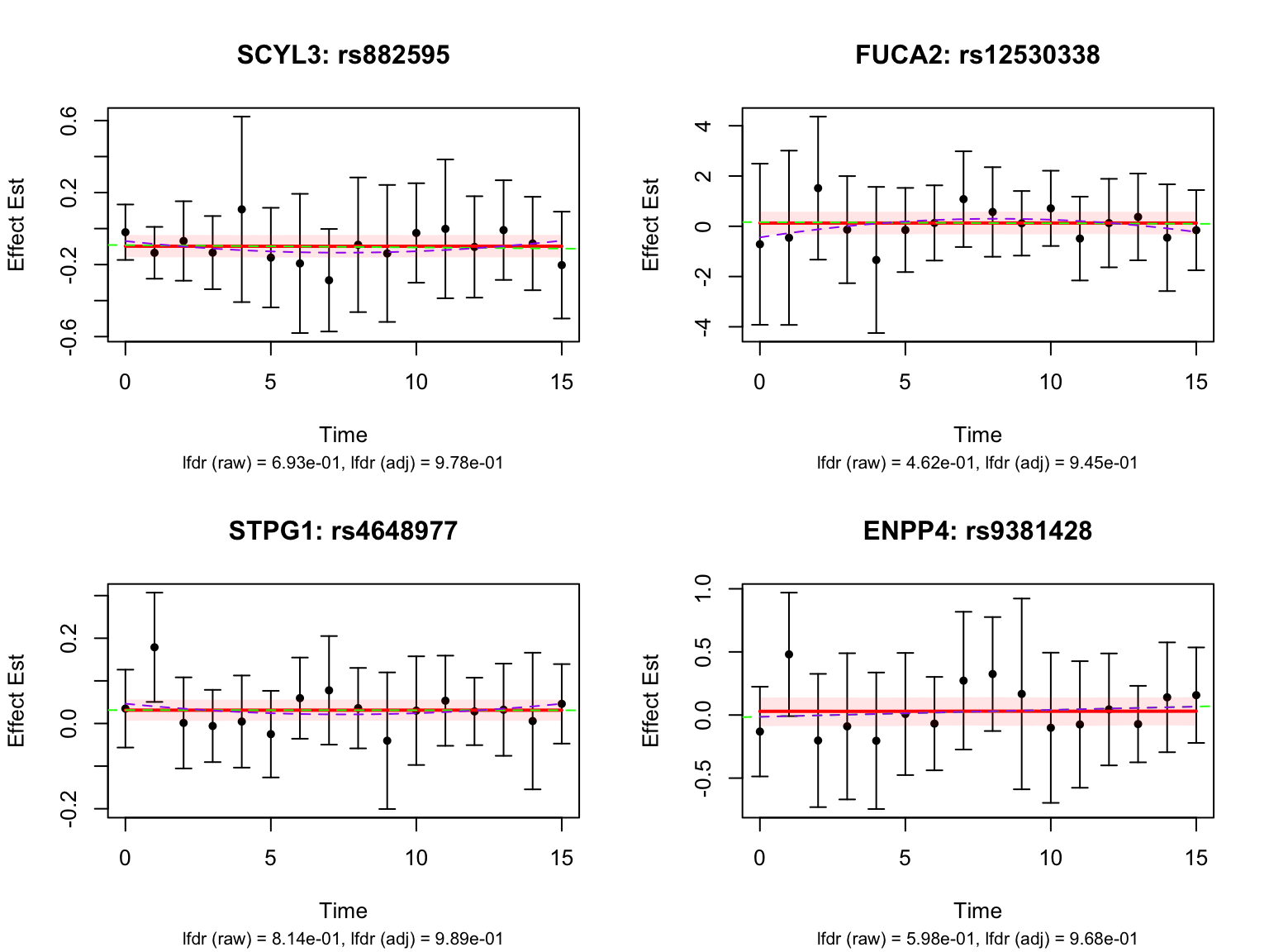
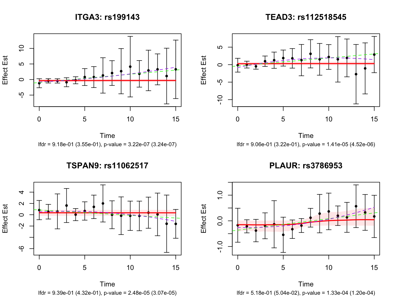
Visualize top-ranked pairs for some selected genes:
Some examples of null pairs:
Comparing with Strober et.al
We will compare the detected dynamic eQTLs with the results from Strober et.al.
What are the p-value cutoff for linear and non-linear methods in Strober et.al?
pval_cutoff_strober_nonlinear <- max(strober_nonlinear_highlighted$pvalue)
pval_cutoff_strober_linear <- max(strober_linear_highlighted$pvalue)
pval_cutoff_strober_nonlinear
[1] 6.829826e-05pval_cutoff_strober_linear[1] 0.0001702417What are the lfdr cutoff for FASH (order 1) before and after BF adjustment?
lfdr_cutoff1_before <- max(fash_fit1$lfdr[test1$fdr_results$index[test1$fdr_results$FDR <= alpha]])
lfdr_cutoff1_after  <- max(fash_fit1_update$lfdr[test1$fdr_results$index[test1$fdr_results$FDR <= alpha]])
lfdr_cutoff1_before
[1] 0.00856825lfdr_cutoff1_after[1] 0.1474749Let’s take a look at the overlap between the two methods used in Strober et.al and FASH (order 1):
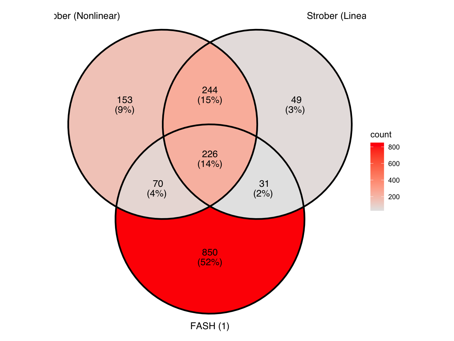
Produce another Venn diagram for the pairs detected by the three methods:
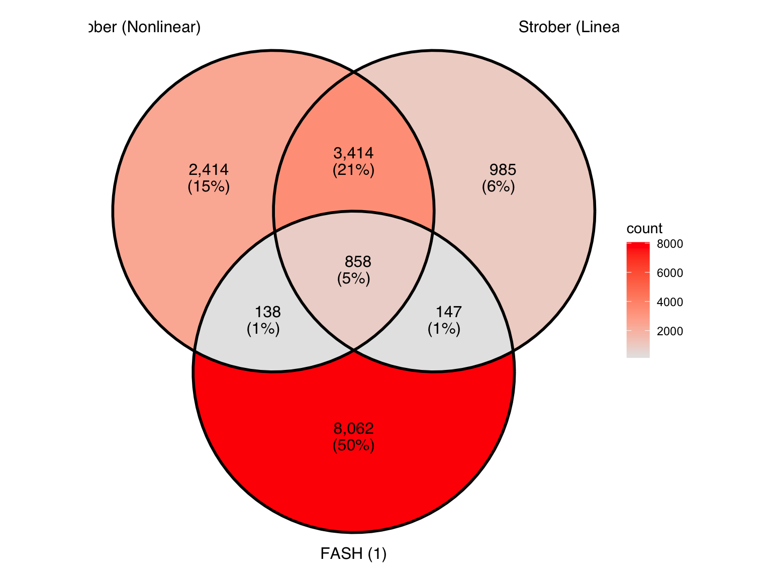
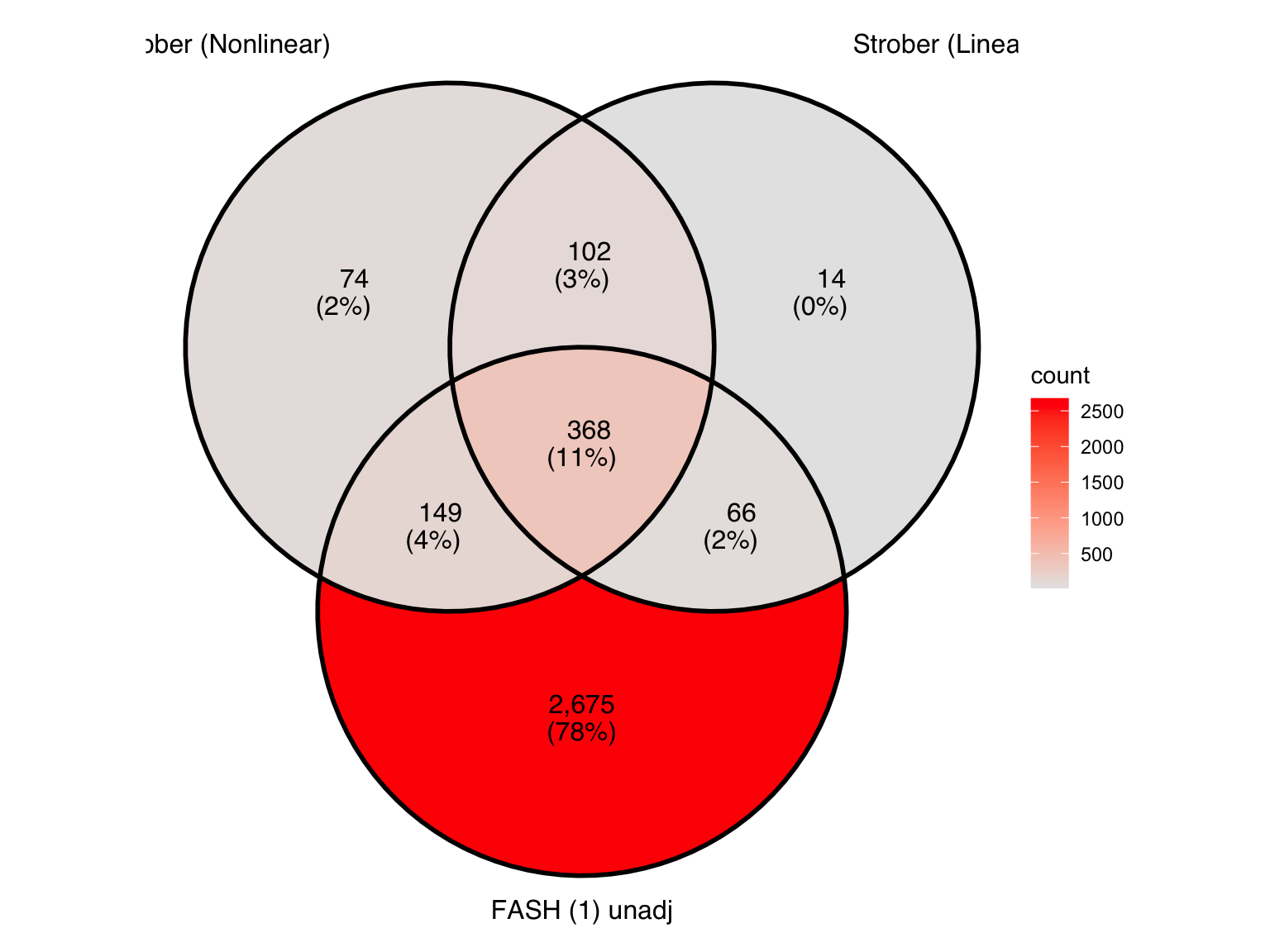
Produce similar Venn diagrams for genes and pairs detected by FASH without BF adjustment:
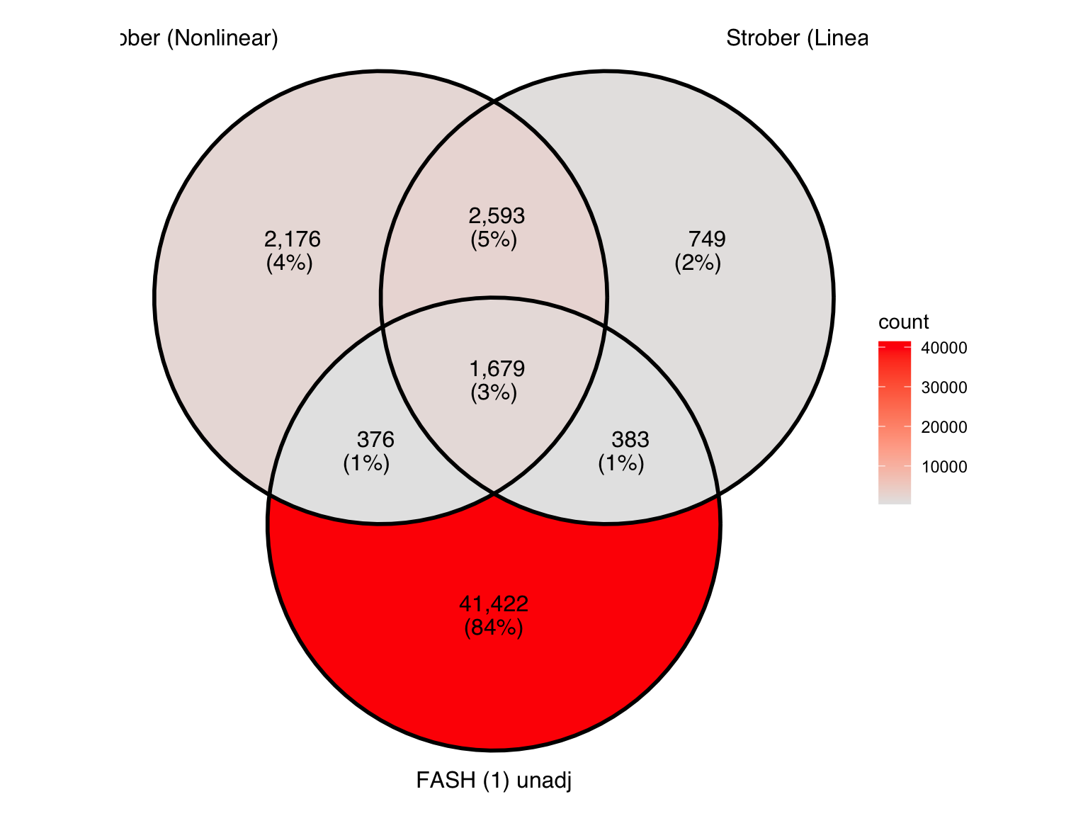
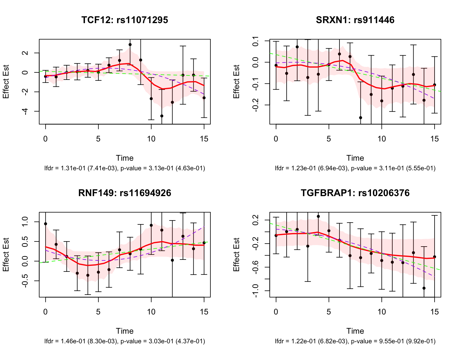
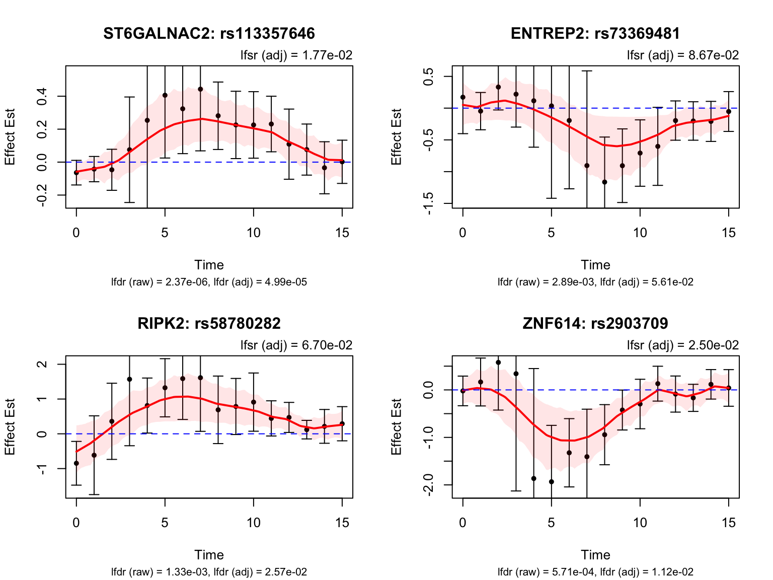
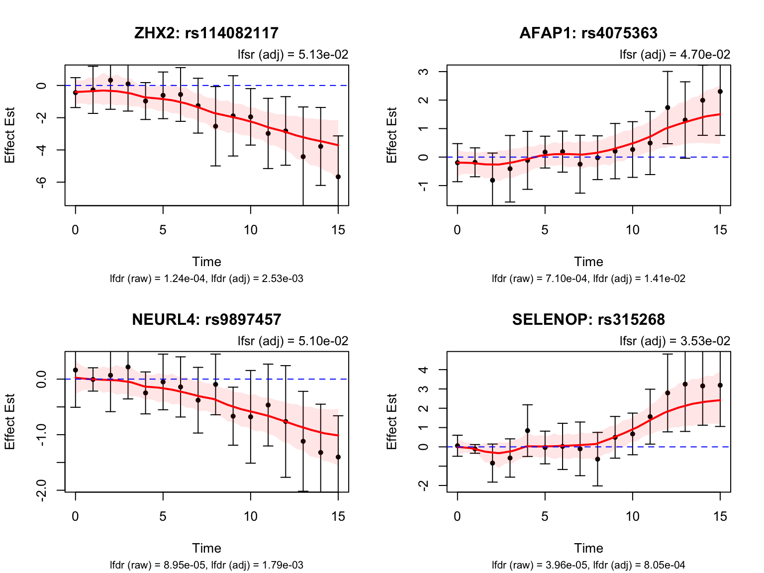
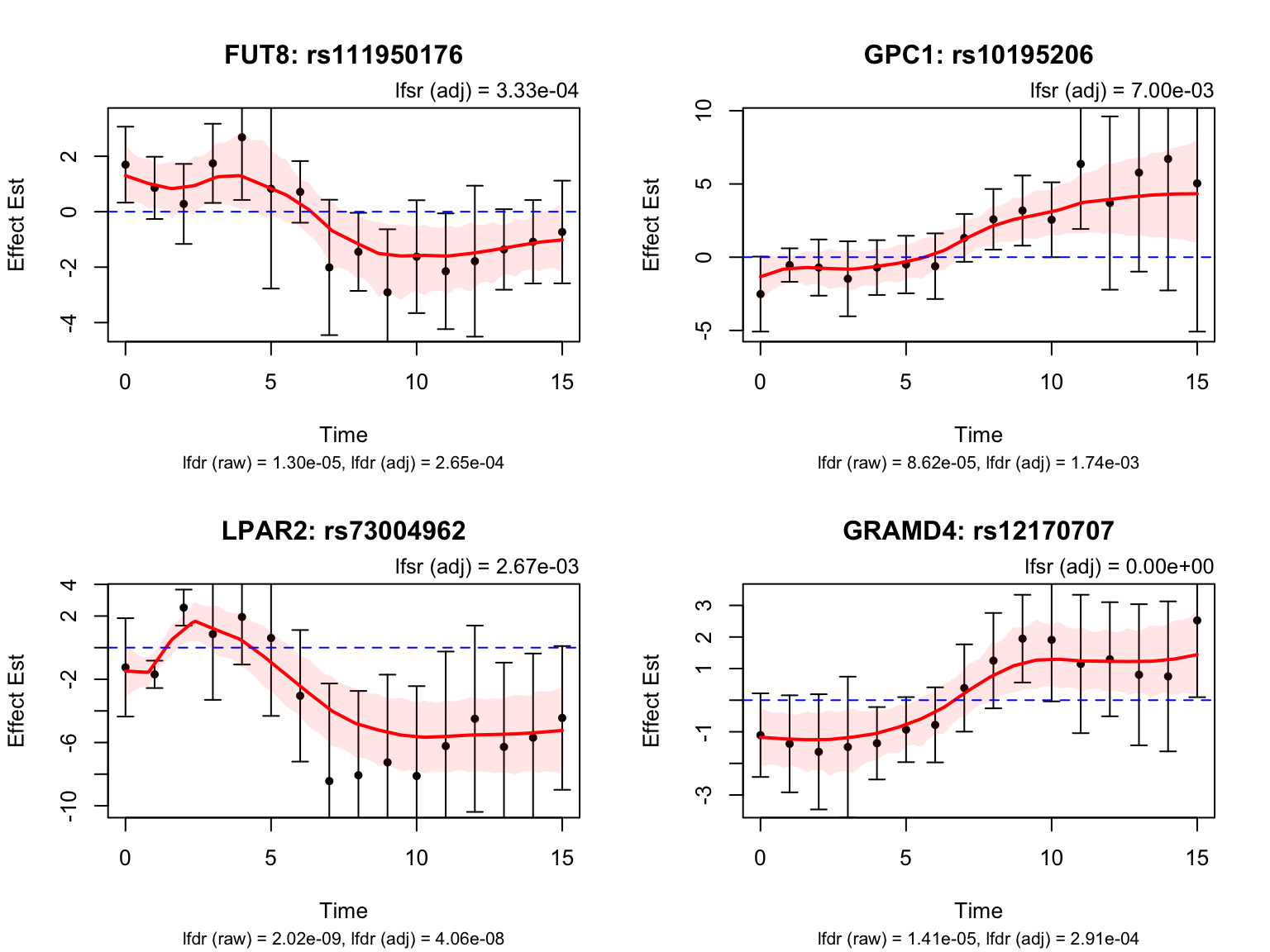
There is a large number of genes only detected by FASH (order 1). Let’s take a look at the 4 pairs that are least significant from FASH, and have at least p-value 0.2 from Strober et.al (both linear and non-linear):
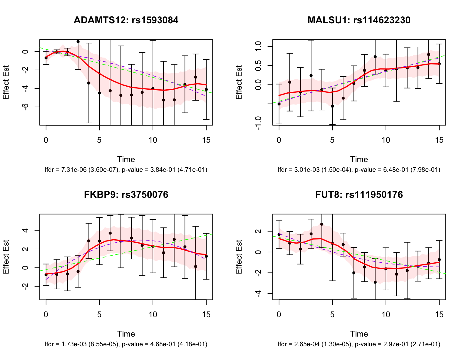
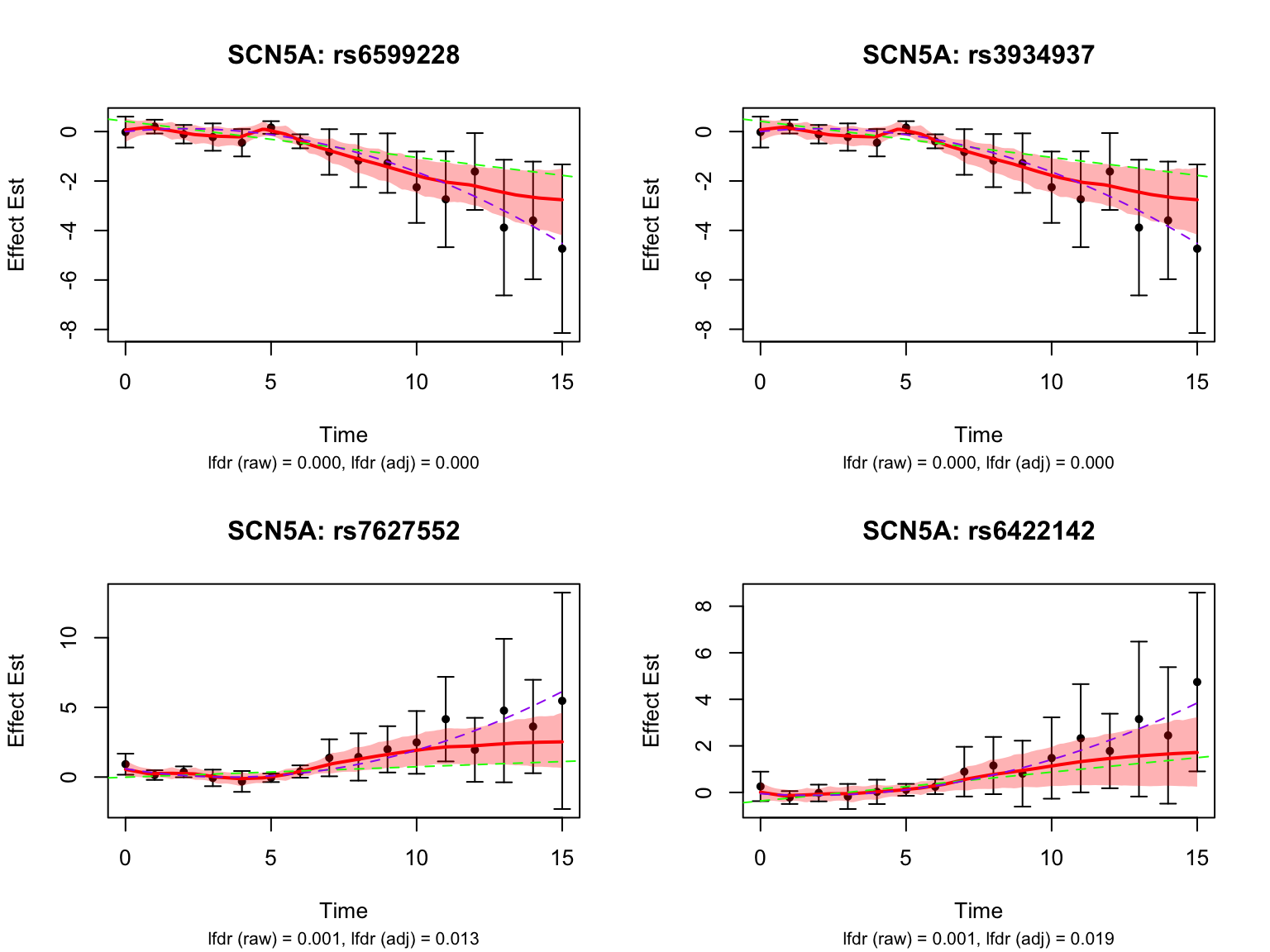
Let’s also take a look at the 4 pairs that are most significant from FASH, also with at least p-value 0.2 from Strober et.al (both linear and non-linear):
Take a look at the p-values and eFDRs from Strober et.al for some of these pairs:
select_gene_id <- gene_map$ensembl_gene_id[gene_map$hgnc_symbol %in% selected_gene_fashr_only]
select_variant_id <- c("rs1593084", "rs114623230", "rs3750076", "rs111950176")

strober_linear %>%
  filter(rs_id %in% select_variant_id, ensamble_id %in% select_gene_id)
# A tibble: 4 × 6
rs_id ensamble_id pvalue eFDR key gene_symbol
<chr> <chr> <dbl> <dbl> <chr> <chr>
1 rs111950176 ENSG00000033170 0.297 0.796 ENSG00000033170_rs111950… FUT8
2 rs1593084 ENSG00000151388 0.384 0.845 ENSG00000151388_rs1593084 ADAMTS12
3 rs3750076 ENSG00000122642 0.468 0.878 ENSG00000122642_rs3750076 FKBP9
4 rs114623230 ENSG00000156928 0.648 0.934 ENSG00000156928_rs114623… MALSU1 strober_nonlinear %>%
filter(rs_id %in% select_variant_id, ensamble_id %in% select_gene_id)# A tibble: 4 × 6
rs_id ensamble_id pvalue eFDR key gene_symbol
<chr> <chr> <dbl> <dbl> <chr> <chr>
1 rs111950176 ENSG00000033170 0.271 0.837 ENSG00000033170_rs111950… FUT8
2 rs3750076 ENSG00000122642 0.418 0.909 ENSG00000122642_rs3750076 FKBP9
3 rs1593084 ENSG00000151388 0.471 0.928 ENSG00000151388_rs1593084 ADAMTS12
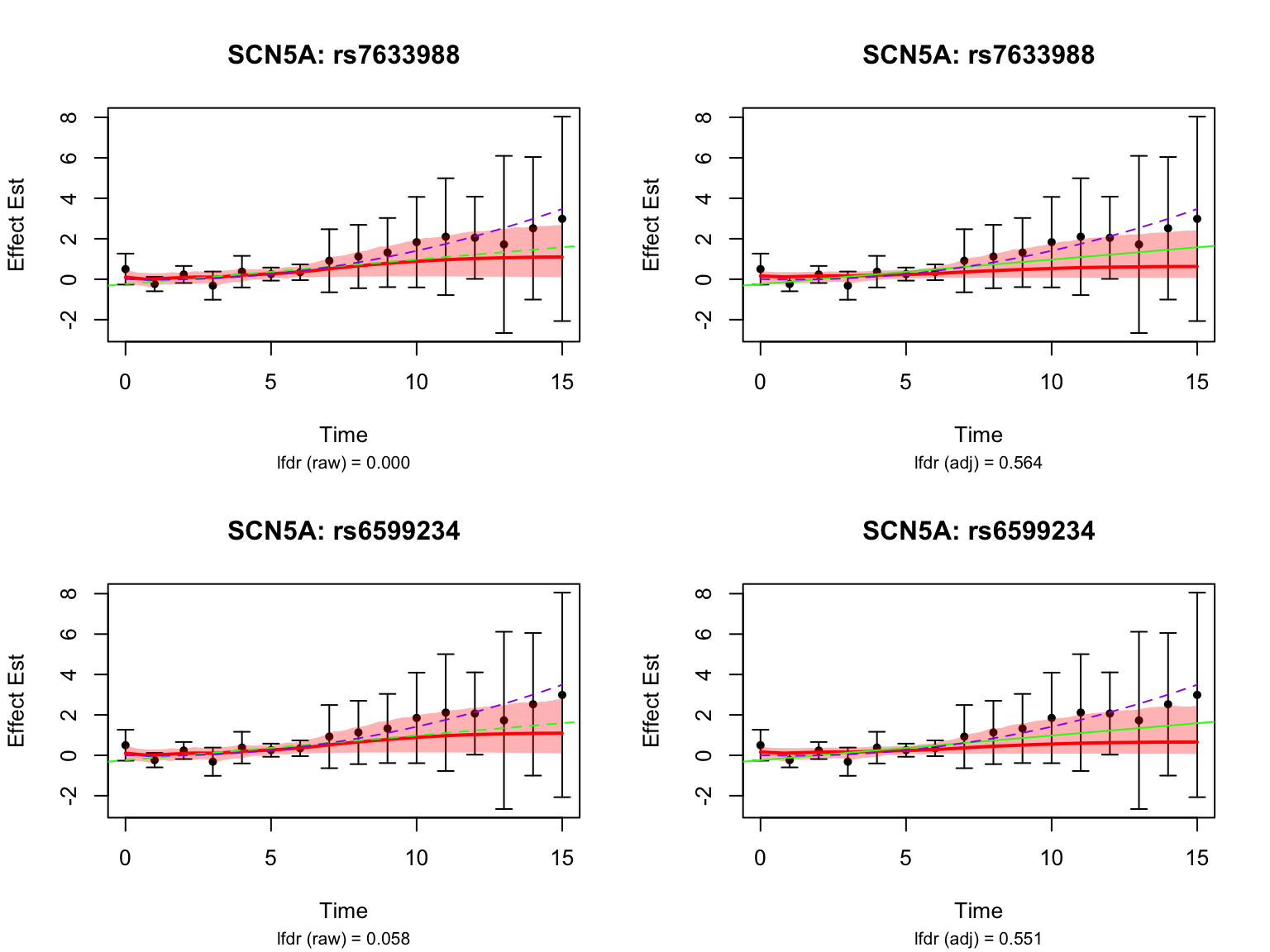
4 rs114623230 ENSG00000156928 0.798 0.986 ENSG00000156928_rs114623… MALSU1 Next, look at some genes that were detected by both FASH and Strober et.al. We will pick the most significant pair for each gene in FASH’s results:
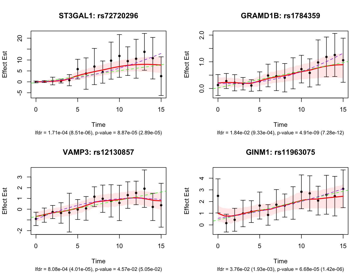
Let’s also look at the genes that were missed by FASH, but detected by Strober et.al. In this case, we will pick the most significant pair for each gene in Strober et.al’s results:
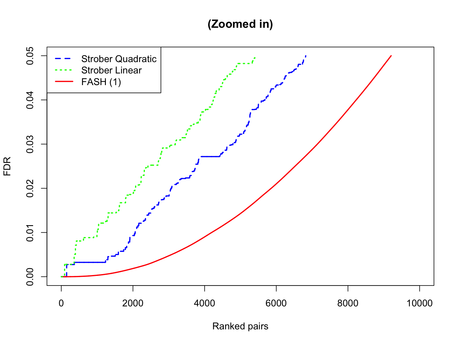
The shape of eFDR (Strober et al) and FDR (FASH):
subset_size <- 10000
subset_seq <- round(seq(1, length(test1$fdr_results$FDR), length.out = subset_size))

plot(
  sort(strober_nonlinear$eFDR)[subset_seq],
  x = subset_seq,
  type = "l",
  col  = "blue",
  lwd  = 2,
  xlab = "Ranked pairs",
  ylab = "FDR",
  lty = "dashed",
  main = ""
)
lines(sort(test1$fdr_results$FDR)[subset_seq], x = subset_seq, col = "red", lty = "solid",  lwd = 2)
lines(sort(strober_linear$eFDR)[subset_seq],   x = subset_seq, col = "green", lty = "dotted", lwd = 2)

legend(
  "topleft",
  legend = c("Strober Quadratic", "Strober Linear", "FASH (1)"),
  col    = c("blue", "green", "red"),
  lty    = c("dashed", "dotted", "solid"),
  lwd    = c(2, 2, 2)
)
plot(
  sort(strober_nonlinear$eFDR[strober_nonlinear$eFDR <= 0.05]),
  xlim = c(0, 10000),
  type = "l",
  col  = "blue",
  lwd  = 2,
  lty  = "dashed",
  xlab = "Ranked pairs",
  ylab = "FDR",
  main = "(Zoomed in)"
)
lines(sort(test1$fdr_results$FDR[test1$fdr_results$FDR <= 0.05]), col = "red",   lty = "solid",  lwd = 2)
lines(sort(strober_linear$eFDR[strober_linear$eFDR <= 0.05]),     col = "green", lty = "dotted", lwd = 2)

legend(
  "topleft",
  legend = c("Strober Quadratic", "Strober Linear", "FASH (1)"),
  col    = c("blue", "green", "red"),
  lty    = c("dashed", "dotted", "solid"),
  lwd    = c(2, 2, 2)
)
Scatterplot of lfdr and p-values from Strober et.al:
fash_tbl <- pair_tbl %>%
  transmute(key, ens_id, rs_id, idx,
            lfdr_raw = fash_fit1$lfdr[idx],
            lfdr_adj = fash_fit1_update$lfdr[idx])

manual_symbol <- c("ENSG00000225485" = "NFATC4")

plot_lfdr_vs_p(
  fash_tbl,
  strober_linear,
  pval_cutoff_strober_linear,
  lfdr_cutoff1_after,
  gene_map,
  title_text = "Scatterplot of lfdr (FASH) vs p-values (Strober Linear)",
  manual_symbol = manual_symbol
)
plot_lfdr_vs_p(
  fash_tbl,
  strober_nonlinear,
  pval_cutoff_strober_nonlinear,
  lfdr_cutoff1_after,
  gene_map,
  title_text = "Scatterplot of lfdr (FASH) vs p-values (Strober Quadratic)",
  manual_symbol = manual_symbol
)
Classifying dynamic eQTLs
Following the definition in Strober et.al, we will classify the detected dynamic eQTLs into different categories:
Early: eQTLs with strongest effect during the first three days: \(\max_{t\leq3} |\beta(t)| - \max_{t> 3} |\beta(t)| > 0\).
Late: eQTLs with strongest effect during the last four days: \(\max_{t\geq 12} |\beta(t)| - \max_{t< 12} |\beta(t)| > 0\).
Middle: eQTLs with strongest effect during days 4-11: \(\max_{4\leq t\leq 11} |\beta(t)| - \max_{t> 11 | t< 4} |\beta(t)| > 0\).
Switch: eQTLs with effect sign switch during the time course such that \(\min\{\max\beta(t)^+,\max\beta(t)^-\}-c>0\) where \(c\) is a threshold that we set to 0.25 (which means with two alleles, the maximal difference of effect size is at least \(\geq 2\times\min\{\max\beta(t)^+,\max\beta(t)^-\}\times2 \geq 2 \times 0.25 \times 2 = 1\)).
We will take a look at the significant pairs detected by FASH (order 1), and classify them based on the false sign rate (lfsr).
Early dynamic eQTLs
smooth_var_refined = seq(0,15, by = 0.1)
functional_early <- function(x){
  max(abs(x[smooth_var_refined <= 3])) - max(abs(x[smooth_var_refined > 3]))
}
testing_early_dyn <- testing_functional(functional_early,
                                              lfsr_cal = function(x){mean(x <= 0)},
                                              fash = fash_fit1,
                                              indices = fash_highlighted1,
                                              smooth_var = smooth_var_refined)
How many pairs and how many unique genes are classified as early dynamic eQTLs?
load(file.path(result_dir, "classify_dyn_eQTLs_early.RData"))
early_indices <- testing_early_dyn$indices[testing_early_dyn$cfsr <= alpha]
length(early_indices)
[1] 124early_genes <- unique(pair_tbl$ens_id[pair_tbl$idx %in% early_indices])
length(early_genes)[1] 8Let’s take a look at the top-ranked early dynamic eQTLs:
Middle dynamic eQTLs
functional_middle <- function(x){
  max(abs(x[smooth_var_refined <= 11 & smooth_var_refined >= 4])) - max(abs(x[smooth_var_refined > 11]), abs(x[smooth_var_refined < 4]))
}
testing_middle_dyn <- testing_functional(functional_middle,
                                               lfsr_cal = function(x){mean(x <= 0)},
                                               fash = fash_fit1,
                                               indices = fash_highlighted1,
                                               num_cores = num_cores,
                                               smooth_var = smooth_var_refined)
How many pairs and how many unique genes are classified as middle dynamic eQTLs?
load(file.path(result_dir, "classify_dyn_eQTLs_middle.RData"))
middle_indices <- testing_middle_dyn$indices[testing_middle_dyn$cfsr <= alpha]
length(middle_indices)
[1] 24middle_genes <- unique(pair_tbl$ens_id[pair_tbl$idx %in% middle_indices])
length(middle_genes)[1] 5Take a look at their results:
Late dynamic eQTLs
functional_late <- function(x){
  max(abs(x[smooth_var_refined >= 12])) - max(abs(x[smooth_var_refined < 12]))
}
testing_late_dyn <- testing_functional(functional_late,
                                             lfsr_cal = function(x){mean(x <= 0)},
                                             fash = fash_fit1,
                                             indices = fash_highlighted1,
                                             num_cores = num_cores,
                                             smooth_var = smooth_var_refined)
How many pairs and how many unique genes are classified as late dynamic eQTLs?
load(file.path(result_dir, "classify_dyn_eQTLs_late.RData"))
late_indices <- testing_late_dyn$indices[testing_late_dyn$cfsr <= alpha]
length(late_indices)
[1] 20late_genes <- unique(pair_tbl$ens_id[pair_tbl$idx %in% late_indices])
length(late_genes)[1] 12Let’s take a look at the top-ranked late dynamic eQTLs:
Switch dynamic eQTLs
How many pairs and how many unique genes are classified as switch dynamic eQTLs?
switch_threshold <- 0.25
functional_switch <- function(x){
  x_pos <- x[x > 0]
  x_neg <- x[x < 0]
  if(length(x_pos) == 0 || length(x_neg) == 0){
    return(0)
  }
  min(max(abs(x_pos)), max(abs(x_neg))) - switch_threshold
}
testing_switch_dyn <- testing_functional(functional_switch,
                                               lfsr_cal = function(x){mean(x <= 0)},
                                               fash = fash_fit1,
                                               indices = fash_highlighted1,
                                               num_cores = num_cores,
                                               smooth_var = smooth_var_refined)
load(file.path(result_dir, "classify_dyn_eQTLs_switch.RData"))
switch_indices <- testing_switch_dyn$indices[testing_switch_dyn$cfsr <= alpha]
length(switch_indices)[1] 984switch_genes <- unique(pair_tbl$ens_id[pair_tbl$idx %in% switch_indices])
length(switch_genes)[1] 250Let’s take a look at the top-ranked switch dynamic eQTLs:
Gene Set Enrichment Analysis
library(clusterProfiler)
library(tidyverse)
library(msigdbr)
library(org.Hs.eg.db)
library(cowplot)

m_t2g <- msigdbr(species = "Homo sapiens", category = "H") %>%
  mutate(ensembl_use = dplyr::coalesce(ensembl_gene, db_ensembl_gene)) %>%
  dplyr::filter(!is.na(ensembl_use)) %>%
  dplyr::select(gs_name, ensembl_use) %>%
  dplyr::distinct()

enrich_set <- function(genes_selected,
                       background_gene,
                       q_val_cutoff = 0.05,
                       pvalueCutoff = 0.05) {

  genes_selected_raw  <- unique(as.character(genes_selected))
  background_gene_raw <- unique(as.character(background_gene))

  universe_for_test <- background_gene_raw
  hallmark_genes <- unique(m_t2g$ensembl_use)
  bg_not_in_hallmark <- setdiff(universe_for_test, hallmark_genes)

  dummy_id <- "__DUMMY_BACKGROUND__"

  if (length(bg_not_in_hallmark) > 0) {
    dummy_t2g <- tibble(
      gs_name     = dummy_id,
      ensembl_use = bg_not_in_hallmark
    )
    TERM2GENE_full <- bind_rows(m_t2g, dummy_t2g)
  } else {
    TERM2GENE_full <- m_t2g
  }

  genes_sel_used <- intersect(genes_selected_raw, universe_for_test)

  enrich_res <- enricher(
    gene          = genes_sel_used,
    TERM2GENE     = TERM2GENE_full,
    universe      = universe_for_test,
    pAdjustMethod = "BH",
    qvalueCutoff  = q_val_cutoff,
    pvalueCutoff  = pvalueCutoff
  )

  if (is.null(enrich_res) || nrow(enrich_res@result) == 0L) {
    return(enrich_res)
  }

  df <- enrich_res@result
  df <- df %>% dplyr::filter(ID != dummy_id)

  df$GeneRatio_orig <- df$GeneRatio
  df$BgRatio_orig   <- df$BgRatio

  n_sel_total <- length(genes_sel_used)
  n_bg_total  <- length(universe_for_test)

  df$GeneRatio_fixed <- paste0(df$Count,   "/", n_sel_total)
  df$BgRatio_fixed   <- paste0(df$setSize, "/", n_bg_total)

  enrich_res@result <- df
  enrich_res
}
Among all the genes highlighted by FASH:
result <- enrich_set(genes_selected = genes_highlighted1, background_gene = all_genes)
result@result %>%
  filter(pvalue < 0.05) %>%
  dplyr::select(GeneRatio, BgRatio, pvalue, qvalue)
GeneRatio BgRatio pvalue qvalue
HALLMARK_HYPOXIA 25/1177 89/6362 0.01692525 0.4356805
HALLMARK_IL6_JAK_STAT3_SIGNALING 8/1177 21/6362 0.02796398 0.4356805
HALLMARK_ESTROGEN_RESPONSE_EARLY 22/1177 82/6362 0.03940505 0.4356805
HALLMARK_ESTROGEN_RESPONSE_LATE 21/1177 79/6362 0.04759267 0.4356805
HALLMARK_ANDROGEN_RESPONSE 16/1177 57/6362 0.04992902 0.4356805Among the genes highlighted by FASH that are classified as early dynamic eQTLs:
result <- enrich_set(genes_selected = early_genes, background_gene = all_genes)
result@result %>%
  filter(pvalue < 0.05) %>%
  dplyr::select(GeneRatio, BgRatio, pvalue, qvalue)
[1] GeneRatio BgRatio pvalue qvalue
<0 rows> (or 0-length row.names)Among the genes highlighted by FASH that are classified as middle dynamic eQTLs:
result <- enrich_set(genes_selected = middle_genes, background_gene = all_genes)
result@result %>%
  filter(pvalue < 0.05) %>%
  dplyr::select(GeneRatio, BgRatio, pvalue, qvalue)
GeneRatio BgRatio pvalue qvalue
HALLMARK_INTERFERON_ALPHA_RESPONSE 1/5 27/6362 0.02104696 0.009425976
HALLMARK_ALLOGRAFT_REJECTION 1/5 36/6362 0.02798330 0.009425976
HALLMARK_INFLAMMATORY_RESPONSE 1/5 43/6362 0.03335100 0.009425976
HALLMARK_INTERFERON_GAMMA_RESPONSE 1/5 56/6362 0.04325667 0.009425976
HALLMARK_TNFA_SIGNALING_VIA_NFKB 1/5 58/6362 0.04477338 0.009425976Among the genes highlighted by FASH that are classified as late dynamic eQTLs:
result <- enrich_set(genes_selected = late_genes, background_gene = all_genes)
result@result %>%
  filter(pvalue < 0.05) %>%
  dplyr::select(GeneRatio, BgRatio, pvalue, qvalue)
GeneRatio BgRatio pvalue qvalue
HALLMARK_INTERFERON_GAMMA_RESPONSE 2/12 56/6362 0.004746675 0.0449685Among the genes highlighted by FASH that are classified as switch dynamic eQTLs:
result <- enrich_set(genes_selected = switch_genes, background_gene = all_genes)
result@result %>%
  filter(pvalue < 0.05) %>%
  dplyr::select(GeneRatio, BgRatio, pvalue, qvalue)
GeneRatio BgRatio pvalue qvalue
HALLMARK_HYPOXIA 11/250 89/6362 0.0006678177 0.02460381
HALLMARK_KRAS_SIGNALING_UP 7/250 47/6362 0.0021770248 0.03482415
HALLMARK_MYOGENESIS 8/250 67/6362 0.0044533220 0.03482415
HALLMARK_P53_PATHWAY 9/250 83/6362 0.0050115531 0.03482415
HALLMARK_GLYCOLYSIS 10/250 100/6362 0.0056547761 0.03482415
HALLMARK_ANDROGEN_RESPONSE 7/250 57/6362 0.0065621240 0.03482415
HALLMARK_COAGULATION 5/250 31/6362 0.0066165891 0.03482415
HALLMARK_IL6_JAK_STAT3_SIGNALING 4/250 21/6362 0.0082150106 0.03783229
HALLMARK_NOTCH_SIGNALING 3/250 15/6362 0.0192133471 0.07865113
HALLMARK_APICAL_JUNCTION 7/250 82/6362 0.0414822992 0.15282952
sessionInfo()R version 4.5.1 (2025-06-13)
Platform: aarch64-apple-darwin20
Running under: macOS Sequoia 15.6.1
Matrix products: default
BLAS: /Library/Frameworks/R.framework/Versions/4.5-arm64/Resources/lib/libRblas.0.dylib
LAPACK: /Library/Frameworks/R.framework/Versions/4.5-arm64/Resources/lib/libRlapack.dylib; LAPACK version 3.12.1
locale:
[1] en_US.UTF-8/en_US.UTF-8/en_US.UTF-8/C/en_US.UTF-8/en_US.UTF-8
time zone: America/Chicago
tzcode source: internal
attached base packages:
[1] stats4 stats graphics grDevices utils datasets methods
[8] base
other attached packages:
[1] cowplot_1.2.0 org.Hs.eg.db_3.21.0 AnnotationDbi_1.70.0
[4] IRanges_2.42.0 S4Vectors_0.46.0 Biobase_2.68.0
[7] BiocGenerics_0.54.1 generics_0.1.4 msigdbr_25.1.1
[10] clusterProfiler_4.16.0 lubridate_1.9.4 forcats_1.0.1
[13] readr_2.1.6 tibble_3.3.0 tidyverse_2.0.0
[16] ggVennDiagram_1.5.4 ggrepel_0.9.6 ggplot2_4.0.1
[19] purrr_1.2.0 stringr_1.6.0 tidyr_1.3.1
[22] dplyr_1.1.4 fashr_0.1.42 workflowr_1.7.2
loaded via a namespace (and not attached):
[1] RColorBrewer_1.1-3 rstudioapi_0.17.1 jsonlite_2.0.0
[4] magrittr_2.0.4 ggtangle_0.0.9 farver_2.1.2
[7] rmarkdown_2.30 fs_1.6.6 vctrs_0.6.5
[10] memoise_2.0.1 ggtree_3.16.3 mixsqp_0.3-54
[13] htmltools_0.5.9 curl_7.0.0 gridGraphics_0.5-1
[16] sass_0.4.10 bslib_0.9.0 plyr_1.8.9
[19] cachem_1.1.0 TMB_1.9.19 whisker_0.4.1
[22] igraph_2.2.1 lifecycle_1.0.4 pkgconfig_2.0.3
[25] gson_0.1.0 Matrix_1.7-4 R6_2.6.1
[28] fastmap_1.2.0 GenomeInfoDbData_1.2.14 digest_0.6.39
[31] numDeriv_2016.8-1.1 aplot_0.2.9 enrichplot_1.28.4
[34] colorspace_2.1-2 patchwork_1.3.2 ps_1.9.1
[37] rprojroot_2.1.1 irlba_2.3.5.1 RSQLite_2.4.5
[40] labeling_0.4.3 timechange_0.3.0 httr_1.4.7
[43] compiler_4.5.1 bit64_4.6.0-1 withr_3.0.2
[46] S7_0.2.1 BiocParallel_1.42.2 DBI_1.2.3
[49] R.utils_2.13.0 rappdirs_0.3.3 tools_4.5.1
[52] otel_0.2.0 ape_5.8-1 httpuv_1.6.16
[55] R.oo_1.27.1 glue_1.8.0 callr_3.7.6
[58] nlme_3.1-168 GOSemSim_2.34.0 promises_1.5.0
[61] grid_4.5.1 getPass_0.2-4 reshape2_1.4.5
[64] fgsea_1.34.2 gtable_0.3.6 tzdb_0.5.0
[67] R.methodsS3_1.8.2 data.table_1.17.8 hms_1.1.4
[70] utf8_1.2.6 XVector_0.48.0 pillar_1.11.1
[73] babelgene_22.9 yulab.utils_0.2.3 later_1.4.4
[76] splines_4.5.1 treeio_1.32.0 lattice_0.22-7
[79] bit_4.6.0 tidyselect_1.2.1 GO.db_3.21.0
[82] Biostrings_2.76.0 knitr_1.50 git2r_0.36.2
[85] xfun_0.55 LaplacesDemon_16.1.6 stringi_1.8.7
[88] UCSC.utils_1.4.0 lazyeval_0.2.2 ggfun_0.2.0
[91] yaml_2.3.12 evaluate_1.0.5 codetools_0.2-20
[94] qvalue_2.40.0 ggplotify_0.1.3 cli_3.6.5
[97] processx_3.8.6 jquerylib_0.1.4 dichromat_2.0-0.1
[100] Rcpp_1.1.0 GenomeInfoDb_1.44.3 png_0.1-8
[103] parallel_4.5.1 assertthat_0.2.1 blob_1.2.4
[106] DOSE_4.2.0 tidytree_0.4.6 scales_1.4.0
[109] crayon_1.5.3 rlang_1.1.6 fastmatch_1.1-6
[112] KEGGREST_1.48.1