SuSiE-RSS UKB
Yuxin Zou
2/18/2021
Last updated: 2021-03-16
Checks: 2 0
Knit directory: dsc_susierss/
This reproducible R Markdown analysis was created with workflowr (version 1.6.2). The Checks tab describes the reproducibility checks that were applied when the results were created. The Past versions tab lists the development history.
Great! Since the R Markdown file has been committed to the Git repository, you know the exact version of the code that produced these results.
Great! You are using Git for version control. Tracking code development and connecting the code version to the results is critical for reproducibility.
The results in this page were generated with repository version 21f4a34. See the Past versions tab to see a history of the changes made to the R Markdown and HTML files.
Note that you need to be careful to ensure that all relevant files for the analysis have been committed to Git prior to generating the results (you can use wflow_publish or wflow_git_commit). workflowr only checks the R Markdown file, but you know if there are other scripts or data files that it depends on. Below is the status of the Git repository when the results were generated:
Ignored files:
    Ignored:    .DS_Store
    Ignored:    .Rhistory
    Ignored:    .Rproj.user/

Untracked files:
    Untracked:  data/susie_convergence_problem.rds
    Untracked:  data/susie_convergence_problem6.rds
    Untracked:  data/susierss_ldref.rds

Unstaged changes:
    Modified:   analysis/susierss_ukb_20210218_example.Rmd
    Deleted:    genotype_dir
Note that any generated files, e.g. HTML, png, CSS, etc., are not included in this status report because it is ok for generated content to have uncommitted changes.
These are the previous versions of the repository in which changes were made to the R Markdown (analysis/susierss_ukb_20210218.Rmd) and HTML (docs/susierss_ukb_20210218.html) files. If you’ve configured a remote Git repository (see ?wflow_git_remote), click on the hyperlinks in the table below to view the files as they were in that past version.
| File | Version | Author | Date | Message |
|---|---|---|---|---|
| Rmd | 21f4a34 | zouyuxin | 2021-03-16 | wflow_publish(“analysis/susierss_ukb_20210218.Rmd”) |
| Rmd | 9b772ae | zouyuxin | 2021-03-16 | update results |
| html | 8f8a528 | zouyuxin | 2021-03-03 | Build site. |
| Rmd | 493f3c8 | zouyuxin | 2021-03-03 | wflow_publish(“analysis/susierss_ukb_20210218.Rmd”) |
| html | f1908f9 | zouyuxin | 2021-03-03 | Build site. |
| Rmd | 872995f | zouyuxin | 2021-03-03 | wflow_publish(“analysis/susierss_ukb_20210218.Rmd”) |
| Rmd | 089610a | zouyuxin | 2021-03-03 | add results |
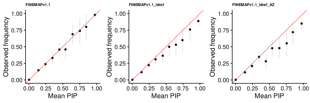
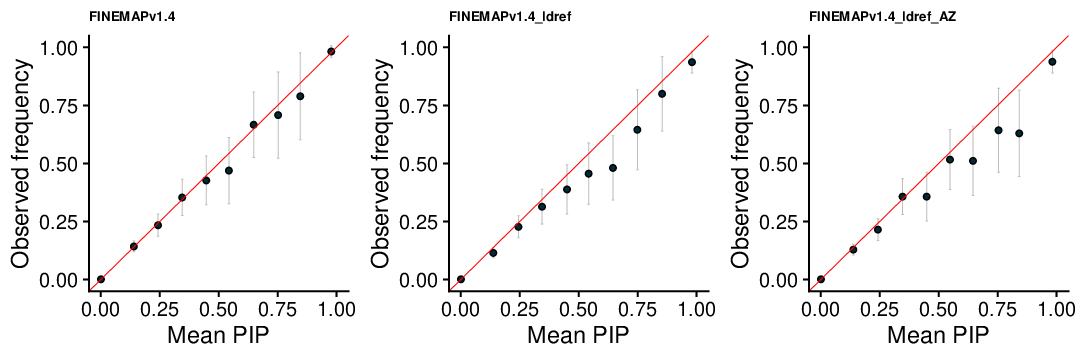
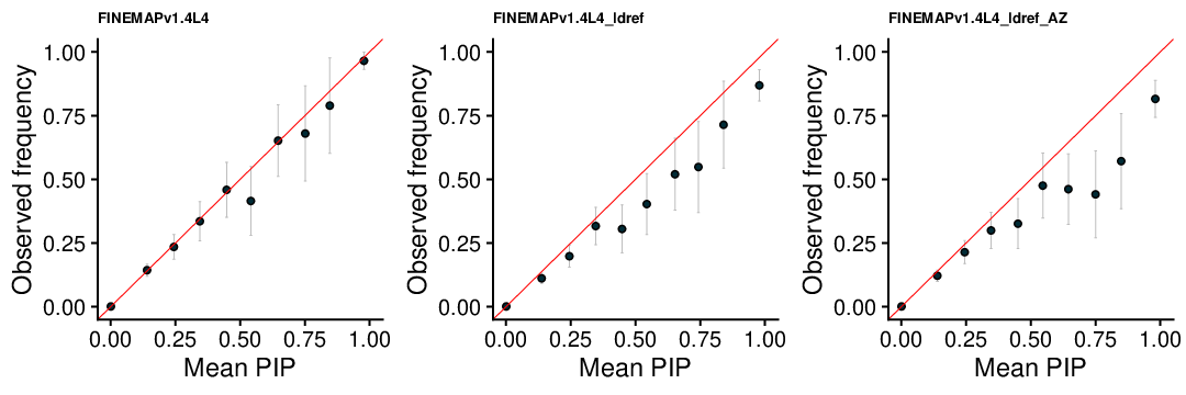
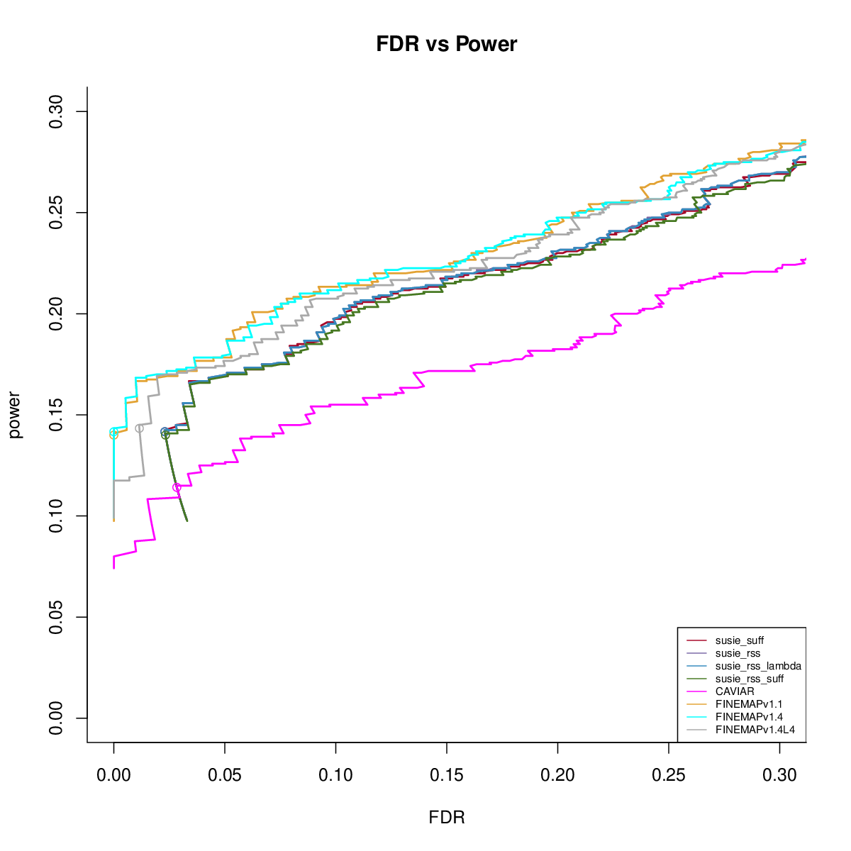
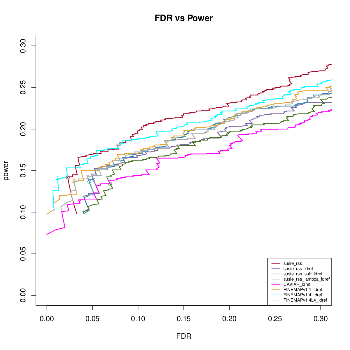
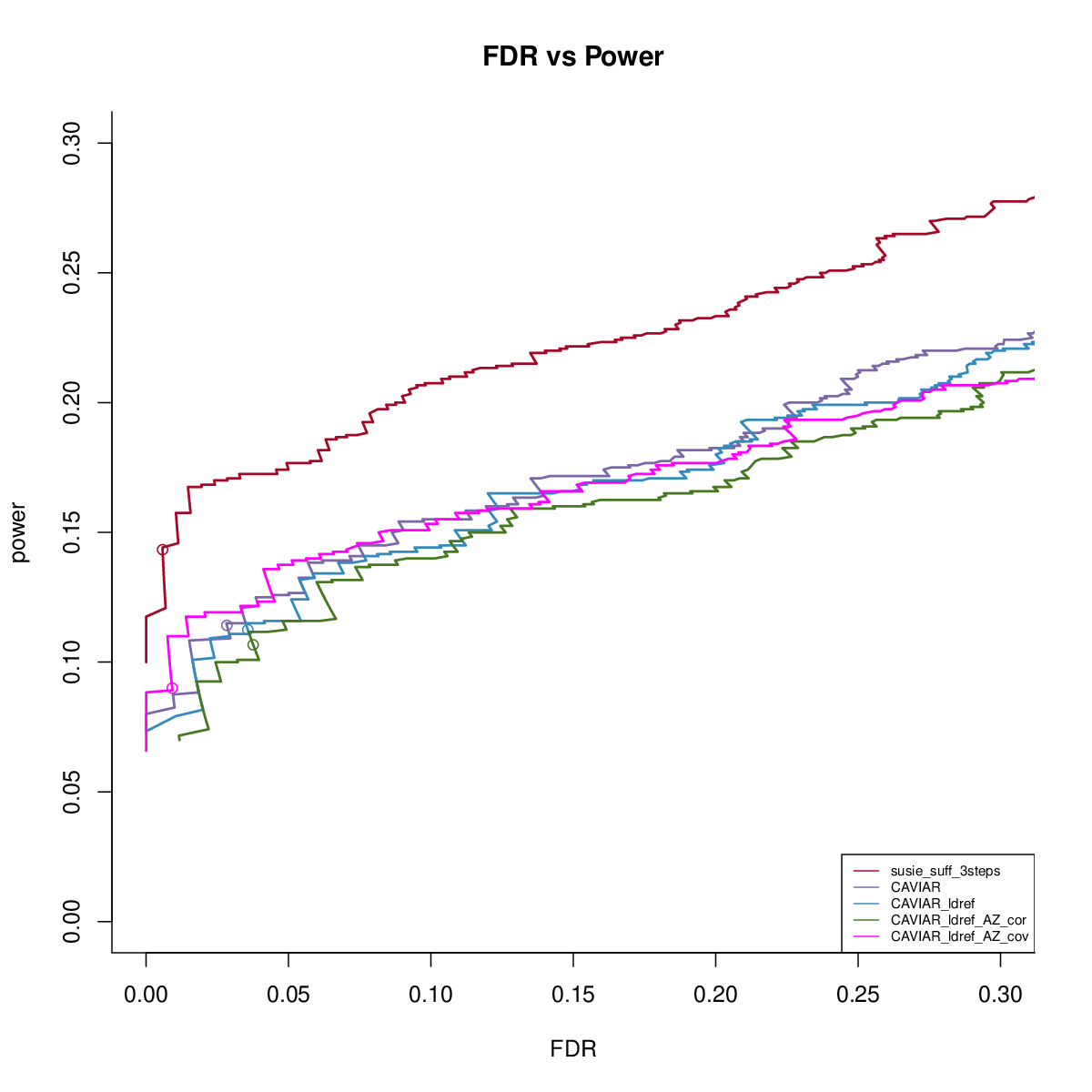
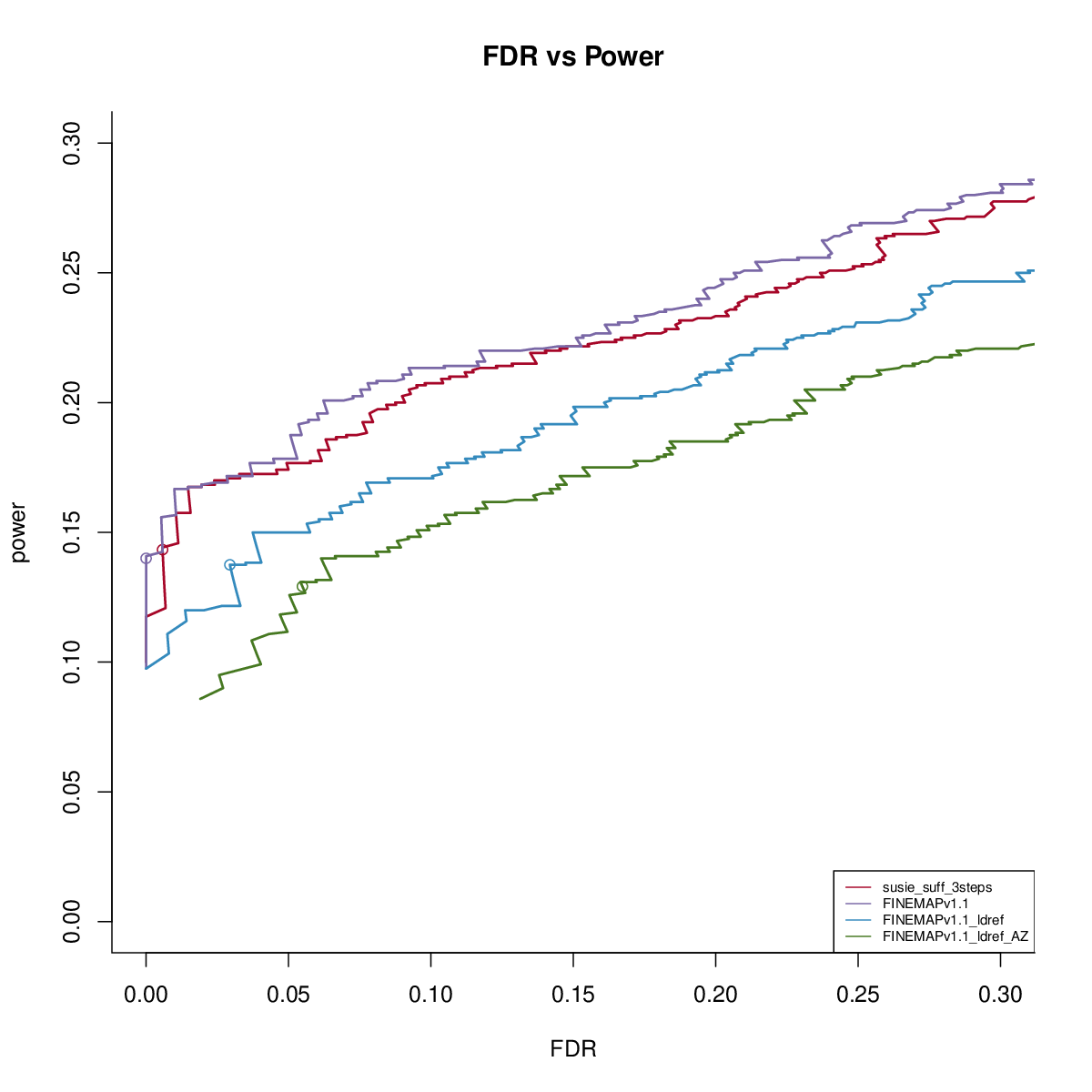
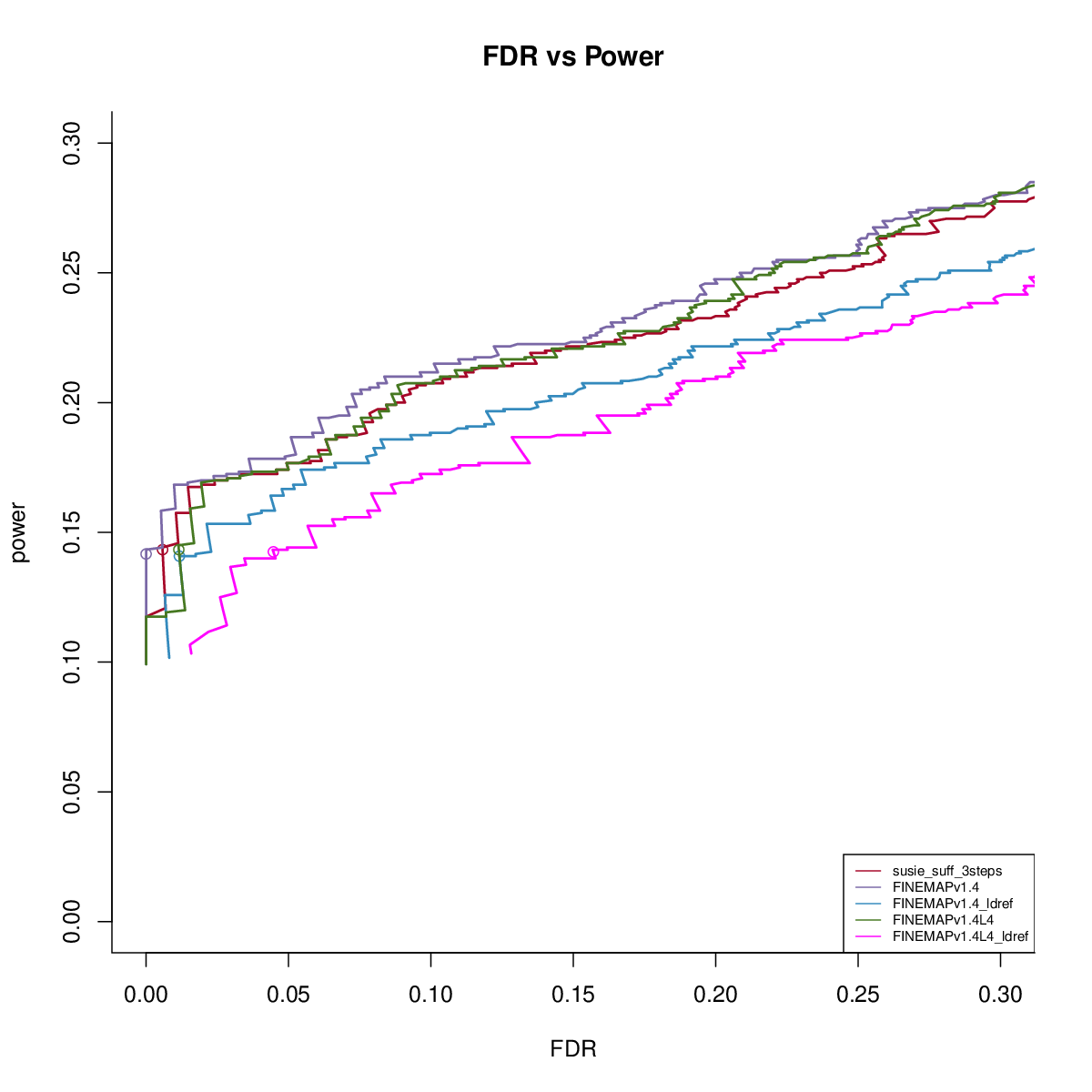
This simulation uses UKB genotype data. We extract the genotype regions based on height GWAS result. There are 200 regions, each with 1000 SNPs. We sample 50,000 individuals to simulate the data. We sample another 1000 samples to get reference LD matrix. We simulate data with 1,2,3 signals and PVE 0.005. We run susie_rss with L=10. We run FINEMAPv1.1 and CAVIAR with oracle number of signals. We run FINEMAPv1.4 with oracle number of signals and max 4 signals.
We first check the impact of estimating residual variance.
The results are similar. We fix residual variance as 1 in the following comparisons.
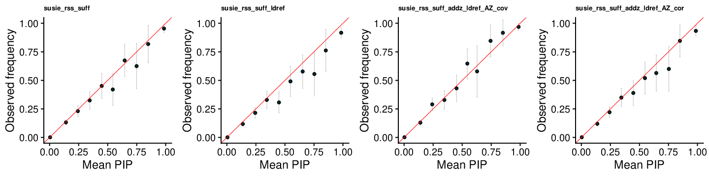
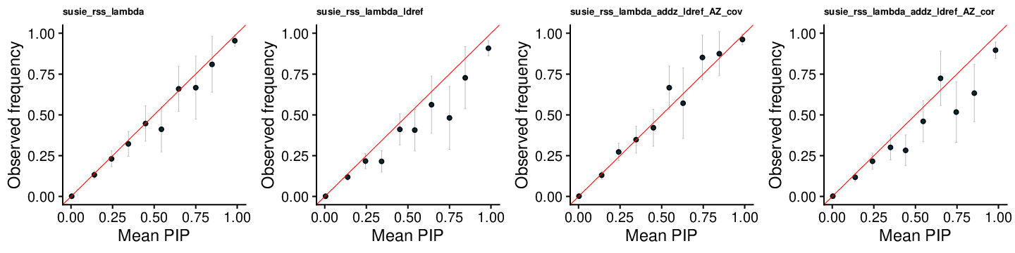
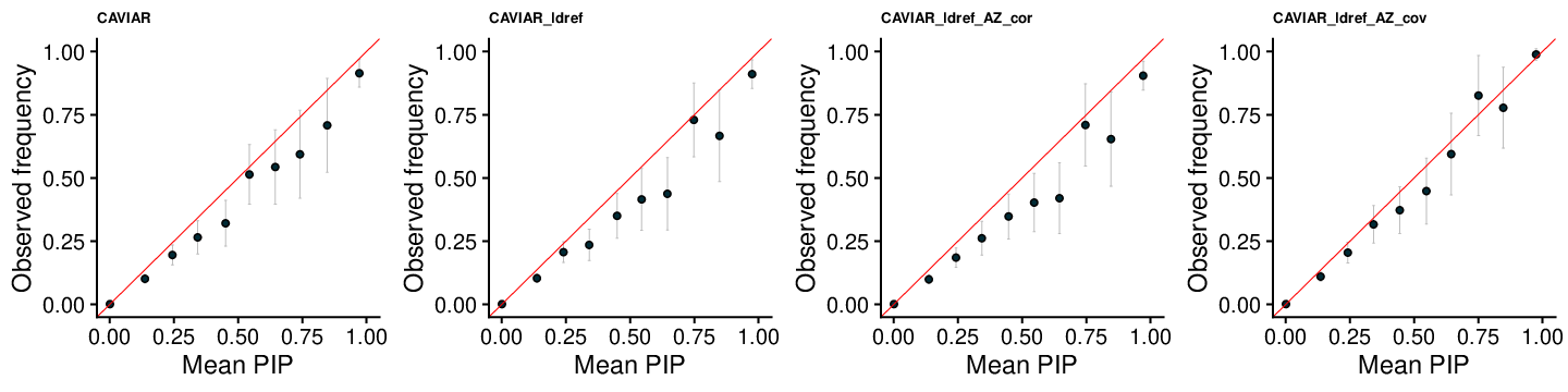
PIP Calibration
SuSiE-RSS
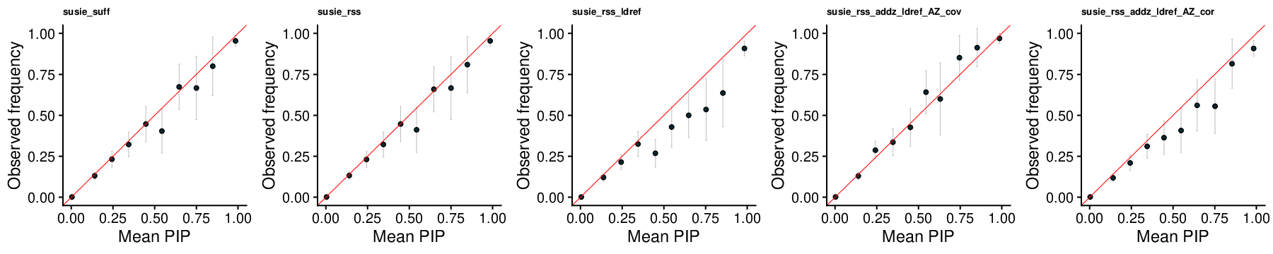
SuSiE-RSS-suff
SuSiE-RSS-lambda
CAVIAR
FINEMAP v1.1
FINEMAP v1.4
FINEMAP v1.4 L4
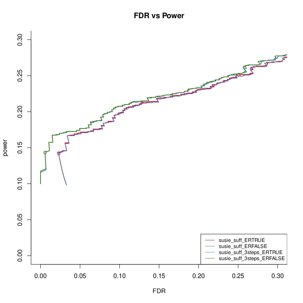
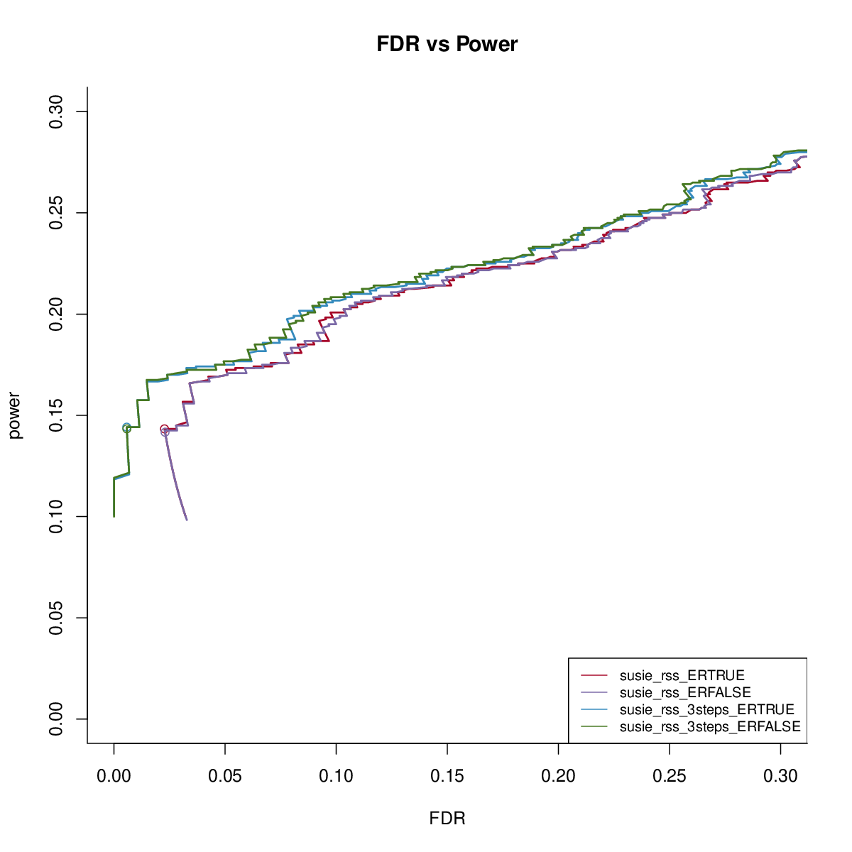
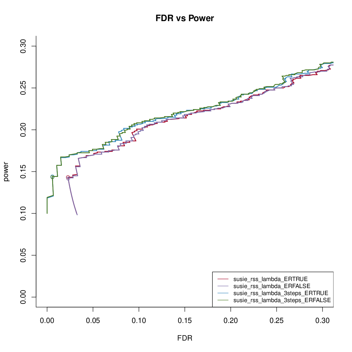
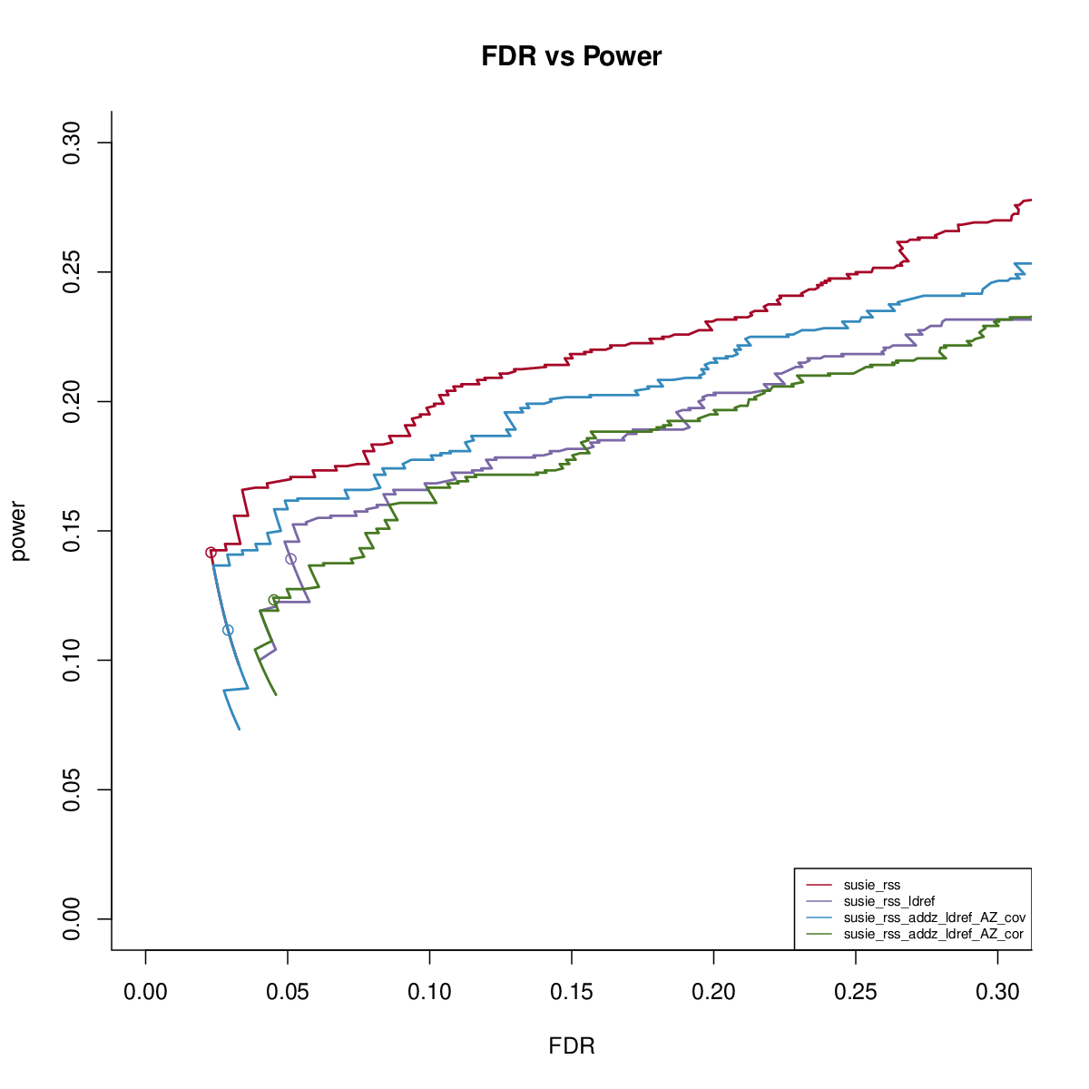
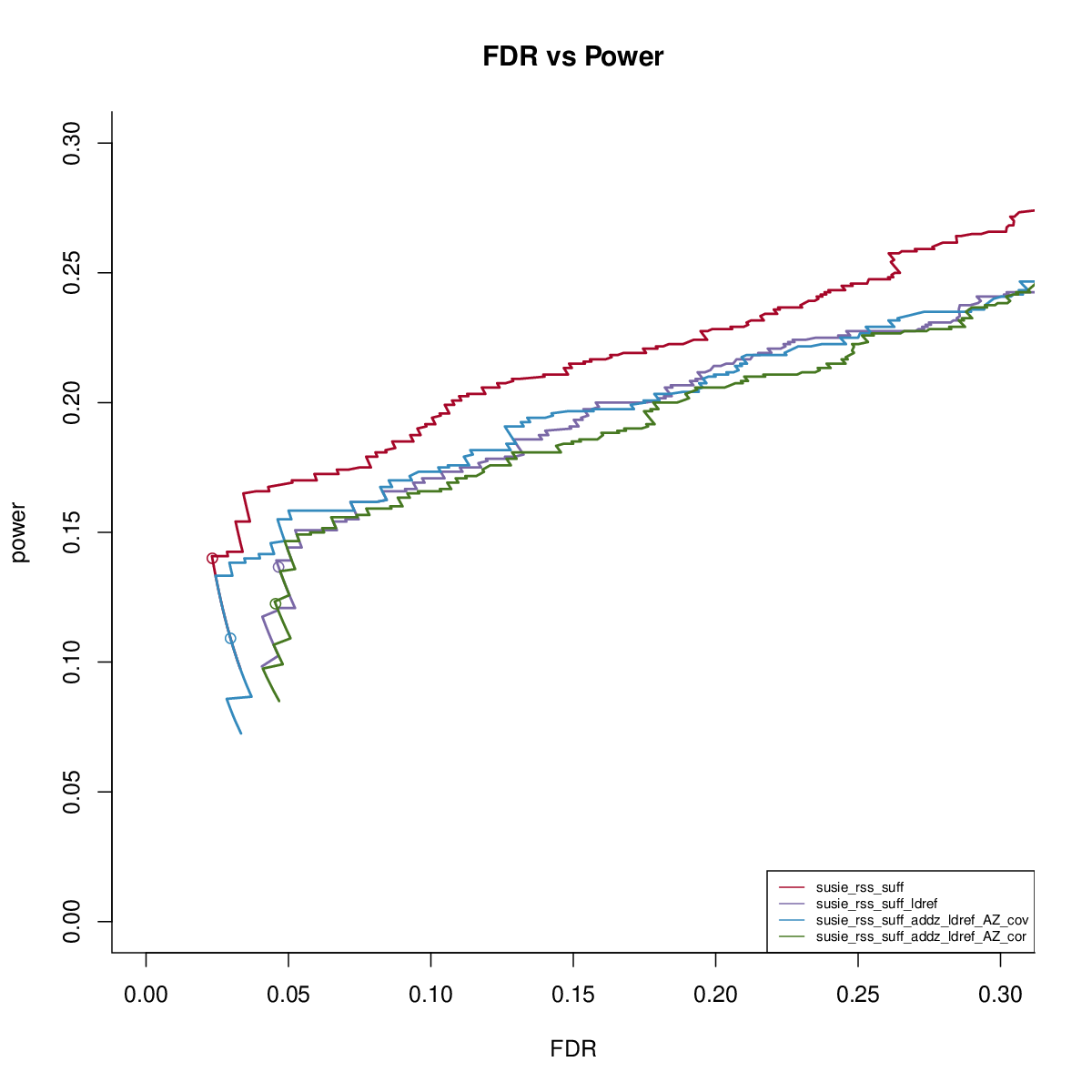
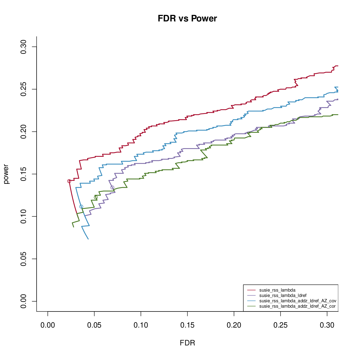
Power vs FDR
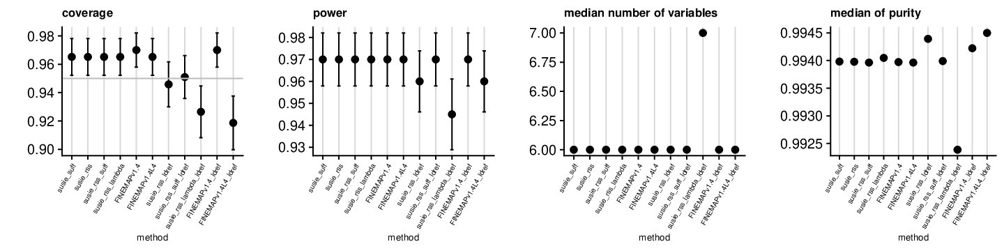
Using in sample LD
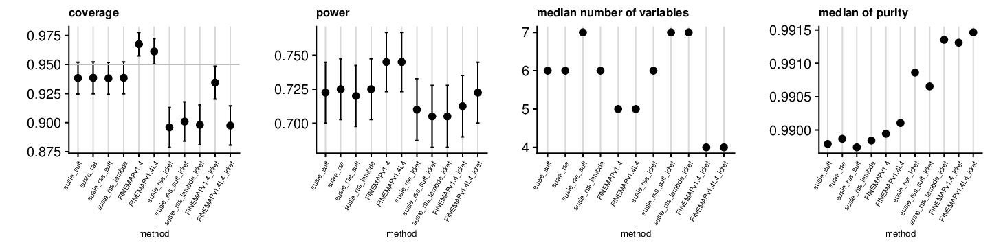
Using ref LD
SuSiE-RSS with reference LD
SuSiE-RSS-suff with reference LD
SuSiE-RSS-lambda with reference LD
CAVIAR with reference LD
FINEMAP v1.1 with reference LD
FINEMAP v1.4 with reference LD
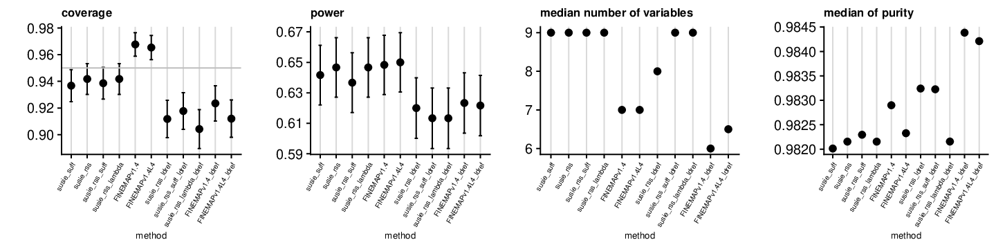
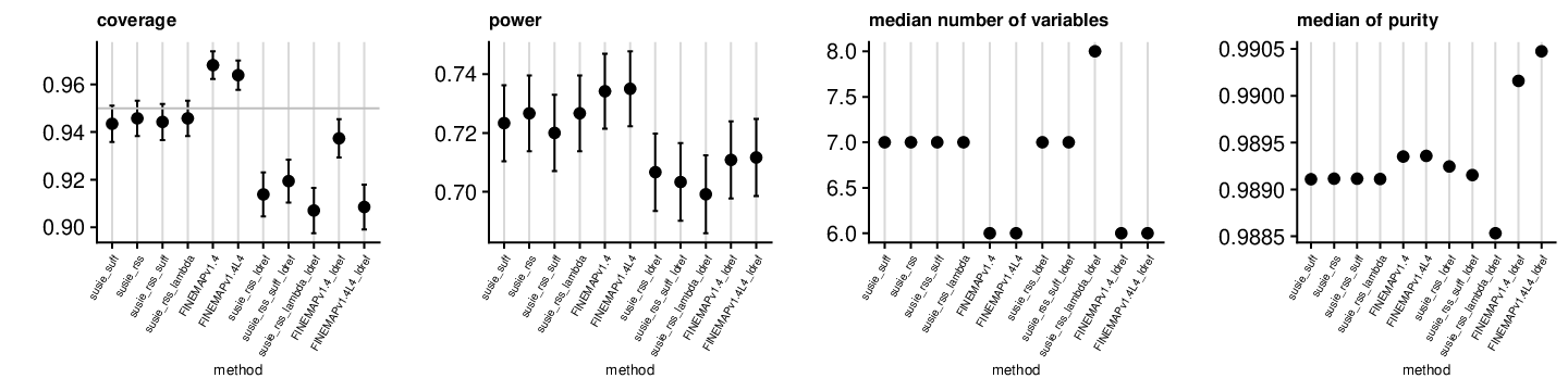
CS
Overall
1 signal
2 signals
3 signals