SuSiE RSS convergence problem

workflowr

• Summary
• Checks
• Past versions

Last updated: 2021-03-09

Checks: 7 0

Knit directory: dsc_susierss/

This reproducible R Markdown analysis was created with workflowr (version 1.6.2). The Checks tab describes the reproducibility checks that were applied when the results were created. The Past versions tab lists the development history.

---

R Markdown file: up-to-date

Great! Since the R Markdown file has been committed to the Git repository, you know the exact version of the code that produced these results.

Environment: empty

Great job! The global environment was empty. Objects defined in the global environment can affect the analysis in your R Markdown file in unknown ways. For reproduciblity it’s best to always run the code in an empty environment.

Seed: set.seed(20210220)

The command set.seed(20210220) was run prior to running the code in the R Markdown file. Setting a seed ensures that any results that rely on randomness, e.g. subsampling or permutations, are reproducible.

Session information: recorded

Great job! Recording the operating system, R version, and package versions is critical for reproducibility.

Cache: none

Nice! There were no cached chunks for this analysis, so you can be confident that you successfully produced the results during this run.

File paths: relative

Great job! Using relative paths to the files within your workflowr project makes it easier to run your code on other machines.

Repository version: b19bb6c

Great! You are using Git for version control. Tracking code development and connecting the code version to the results is critical for reproducibility.

The results in this page were generated with repository version b19bb6c. See the Past versions tab to see a history of the changes made to the R Markdown and HTML files.

Note that you need to be careful to ensure that all relevant files for the analysis have been committed to Git prior to generating the results (you can use wflow_publish or wflow_git_commit). workflowr only checks the R Markdown file, but you know if there are other scripts or data files that it depends on. Below is the status of the Git repository when the results were generated:

Ignored files:
    Ignored:    .DS_Store
    Ignored:    .Rhistory
    Ignored:    .Rproj.user/

Untracked files:
    Untracked:  analysis/susie_ukb_20210307_convergence.Rmd
    Untracked:  data/susie_convergence_problem.rds
    Untracked:  data/susie_convergence_problem6.rds
    Untracked:  data/susierss_ldref.rds

Unstaged changes:
    Modified:   analysis/susierss_ukb_20210218_example.Rmd
    Deleted:    genotype_dir

Note that any generated files, e.g. HTML, png, CSS, etc., are not included in this status report because it is ok for generated content to have uncommitted changes.

---

These are the previous versions of the repository in which changes were made to the R Markdown (analysis/susie_convergence_problem.Rmd) and HTML (docs/susie_convergence_problem.html) files. If you’ve configured a remote Git repository (see ?wflow_git_remote), click on the hyperlinks in the table below to view the files as they were in that past version.

File	Version	Author	Date	Message
Rmd	b19bb6c	zouyuxin	2021-03-09	wflow_publish(“analysis/susie_convergence_problem.Rmd”)
html	5cea1d8	zouyuxin	2021-03-09	Build site.
Rmd	013d610	zouyuxin	2021-03-09	wflow_publish(“analysis/susie_convergence_problem.Rmd”)
html	3d7b065	zouyuxin	2021-03-06	Build site.
Rmd	9fa95fc	zouyuxin	2021-03-06	wflow_publish(“analysis/susie_convergence_problem.Rmd”)
html	53796af	zouyuxin	2021-03-06	Build site.
Rmd	345c9d1	zouyuxin	2021-03-06	wflow_publish(“analysis/susie_convergence_problem.Rmd”)
html	f4fd83c	zouyuxin	2021-03-06	Build site.
Rmd	1e27cc6	zouyuxin	2021-03-06	wflow_publish(“analysis/susie_convergence_problem.Rmd”)
html	065f6f7	zouyuxin	2021-03-06	Build site.
Rmd	fc05b5a	zouyuxin	2021-03-06	wflow_publish(“analysis/susie_convergence_problem.Rmd”)
html	ecaf091	zouyuxin	2021-03-06	Build site.
Rmd	a100dd6	zouyuxin	2021-03-06	wflow_publish(“analysis/susie_convergence_problem.Rmd”)
html	aa199f5	zouyuxin	2021-03-06	Build site.
Rmd	38bddb8	zouyuxin	2021-03-06	wflow_publish(“analysis/susie_convergence_problem.Rmd”)
html	5abf209	zouyuxin	2021-03-06	Build site.
Rmd	311e2c9	zouyuxin	2021-03-06	wflow_publish(“analysis/susie_convergence_problem.Rmd”)
html	9c68be0	zouyuxin	2021-03-06	Build site.
Rmd	8aa8c36	zouyuxin	2021-03-06	wflow_publish(“analysis/susie_convergence_problem.Rmd”)

---

We observe the convergence problem for SuSiE in simulation. We illustrate 3 data here.

For the first one, the default initialization doesn’t work, LASSO initialization works.

For the second one, the default initialization doesn’t work, LASSO initialization doesn’t work.

For the third one, the default initialization works, LASSO initialization doesn’t work.

library(susieR)
dat = readRDS('data/susie_convergence_problem6.rds')

There are 6 data in ‘susie_convergence_problem6.rds’.

Data 1

The region contains 1001 SNPs. There are two causals at 234, 287.

d1 = dat$d1
b = d1$true_coef
idx = which(b!=0)

par(mfrow=c(1,2))
plot(d1$z, pch = 16, xlab = 'SNPs', ylab = 'z')
points(idx, d1$z[idx], col='red', pch = 16)
log10p = -log10(pnorm(-abs(d1$z))*2)
plot(log10p, pch = 16, xlab = 'SNPs', ylab = '-log10 p value')
points(idx, log10p[idx], col='red', pch = 16)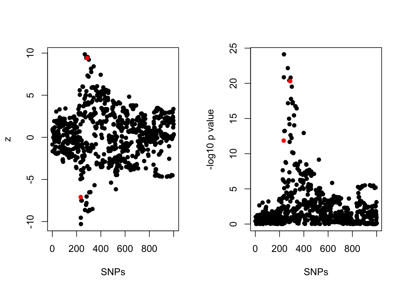

Past versions of unnamed-chunk-2-1.png

Version	Author	Date
9c68be0	zouyuxin	2021-03-06

The SNP with strongest marginal association is 236. The correlation between causal SNPs and top SNP is

cov2cor(d1$XtX)[c(234, 236, 287), c(234, 236, 287)]

             rs4807454_G rs12104241_T rs60120291_A
rs4807454_G    1.0000000   0.56423775   0.53418375
rs12104241_T   0.5642378   1.00000000  -0.03744934
rs60120291_A   0.5341837  -0.03744934   1.00000000

Using L = 3, the susie model gives 3 CSs. (I used susie_suff_stat, which gives the same result as susie.)

f1 = susie_suff_stat(XtX = d1$XtX, Xty = d1$Xty, yty = d1$yty, n = d1$n, L=3, track_fit = T)
susie_plot(f1, y='PIP', b=b, add_legend = T, main=paste0('ELBO: ', round(susie_get_objective(f1), 4)))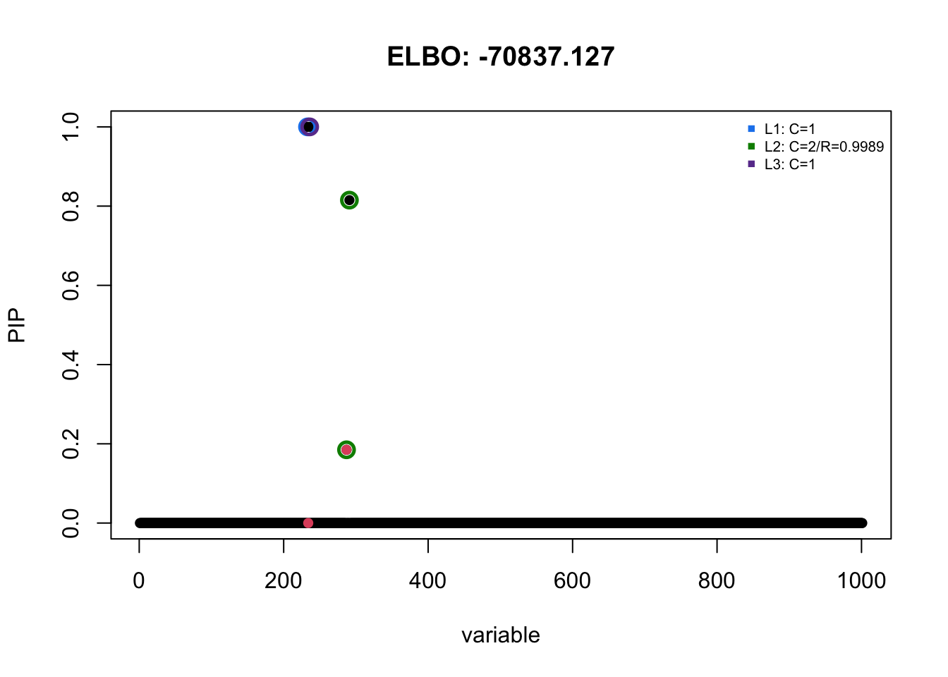

Past versions of unnamed-chunk-4-1.png

Version	Author	Date
9c68be0	zouyuxin	2021-03-06

summary(f1)

Variables in credible sets:

 variable variable_prob cs
      233     1.0000000  3
      236     1.0000000  1
      291     0.8150868  2
      287     0.1849131  2

Credible sets summary:

 cs cs_log10bf cs_avg_r2 cs_min_r2 variable
  1   30.80784 1.0000000 1.0000000      236
  3   31.30944 1.0000000 1.0000000      233
  2   61.20570 0.9989095 0.9978195  287,291

The SNPs in CS1 and CS3 are partially correlated with SNP 234. The correlation between them is

cov2cor(d1$XtX)[c(233, 234, 236), c(233, 234, 236)]

             rs2074944_T rs4807454_G rs12104241_T
rs2074944_T    1.0000000   0.5996649   -0.2407775
rs4807454_G    0.5996649   1.0000000    0.5642378
rs12104241_T  -0.2407775   0.5642378    1.0000000

susie_plot_iteration(f1, L=3, 'assets/susie_convergence_problem/susie_convergence_problem_d1_f1', pos=c(233, 234, 236, 287, 291))

variable	1	2 (C)	3	4 (C)	5
SNP	233	234	236	287	291

knitr::include_graphics("assets/susie_convergence_problem/susie_convergence_problem_d1_f1.gif", error = FALSE)

Past versions of susie_convergence_problem_d1_f1.gif

Version	Author	Date
f97ba78	zouyuxin	2021-03-06

Using L = 2, we find the correct CSs, and the ELBO is larger.

f12 = susie_suff_stat(XtX = d1$XtX, Xty = d1$Xty, yty = d1$yty, n = d1$n, L=2, track_fit = T)
susie_plot(f12, y='PIP', b=b, add_legend = T, main=paste0('ELBO: ', round(susie_get_objective(f12), 3)))

Past versions of unnamed-chunk-9-1.png

Version	Author	Date
065f6f7	zouyuxin	2021-03-06

variable	1	2 (C)	3	4 (C)	5
SNP	233	234	236	287	291

susie_plot_iteration(f12, L=2, 'assets/susie_convergence_problem/susie_convergence_problem_d1_f2', pos=c(233, 234, 236, 287, 291))

knitr::include_graphics("assets/susie_convergence_problem/susie_convergence_problem_d1_f2.gif", error = FALSE)

Past versions of susie_convergence_problem_d1_f2.gif

Version	Author	Date
f97ba78	zouyuxin	2021-03-06

We try to initialize using LASSO solution:

fit.lasso = glmnet::glmnet(d1$X, d1$y, family="gaussian", alpha=1, dfmax = 10)
lasso.b = fit.lasso$beta[,max(which(fit.lasso$df <= 10))]
beta_idx = which(lasso.b != 0)
plot(fit.lasso, label=T)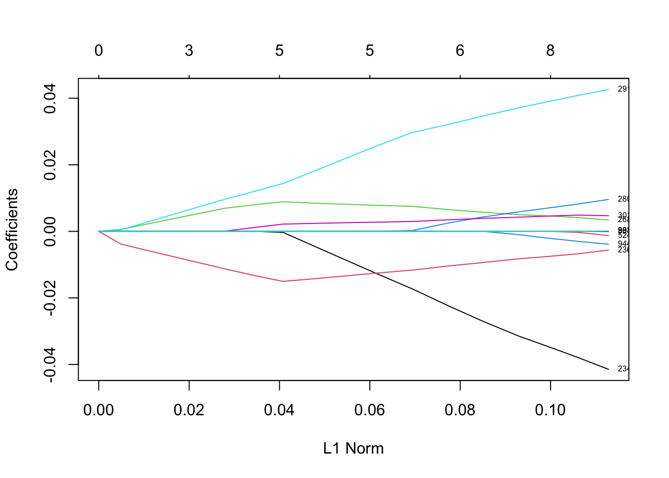

Past versions of unnamed-chunk-12-1.png

Version	Author	Date
f4fd83c	zouyuxin	2021-03-06
065f6f7	zouyuxin	2021-03-06
9c68be0	zouyuxin	2021-03-06

LASSO identifies SNP 234 with non-zero effect, and it doesn’t include SNP 233.

sinit = susieR::susie_init_coef(beta_idx, lasso.b[beta_idx], length(b))
f1lasso = susie_suff_stat(XtX = d1$XtX, Xty = d1$Xty, yty = d1$yty, n = d1$n, s_init = sinit,
                          estimate_residual_variance = T,estimate_prior_variance = TRUE,
                          max_iter = 200, track_fit = T)
susie_plot(f1lasso, y='PIP', b=b, add_legend = T, main=paste0('ELBO: ', round(susie_get_objective(f1lasso), 3)))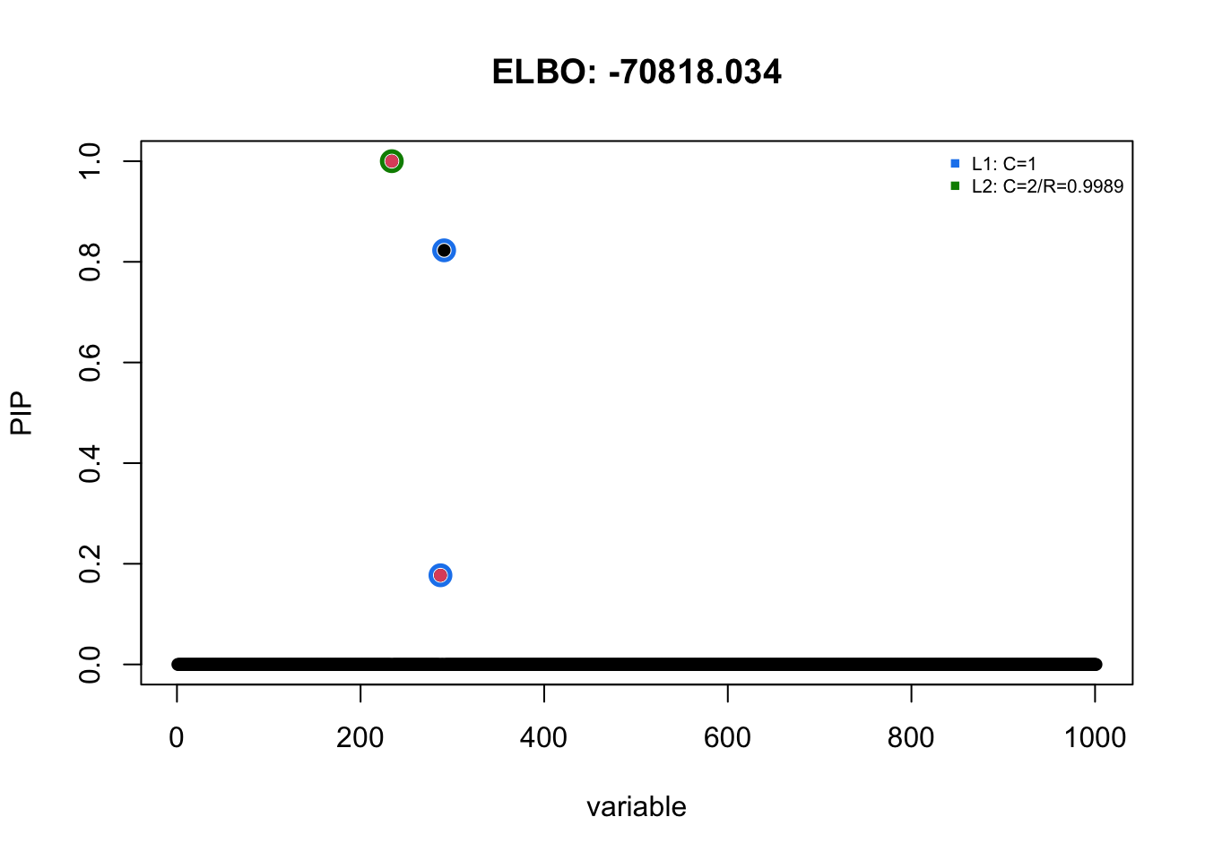

Past versions of unnamed-chunk-13-1.png

Version	Author	Date
f4fd83c	zouyuxin	2021-03-06

We try L0Learn.

library(L0Learn)
set.seed(1)
L0fit = L0Learn.cvfit(d1$X, d1$y, penalty = "L0")
lambdaIndex = which.min(L0fit$cvMeans[[1]]) 
L0coef = as.numeric(coef(L0fit$fit, lambda = L0fit$fit$lambda[[1]][lambdaIndex]))
effect.beta = L0coef[which(L0coef!=0)][-1]
effect.index = (which(L0coef!=0)-1)[-1] 

The effect SNPs are

effect.index

[1] 233 236 291 944

s.init = susie_init_coef(effect.index, effect.beta, length(b))
f1L0.fit = susie_suff_stat(XtX = d1$XtX, Xty = d1$Xty, yty = d1$yty, n = d1$n, s_init = s.init,
                          estimate_residual_variance = T,estimate_prior_variance = TRUE,
                          max_iter = 200, track_fit = T)
susie_plot(f1L0.fit, y='PIP', b=b, add_legend = T, main=paste0('ELBO: ', round(susie_get_objective(f1L0.fit), 3)))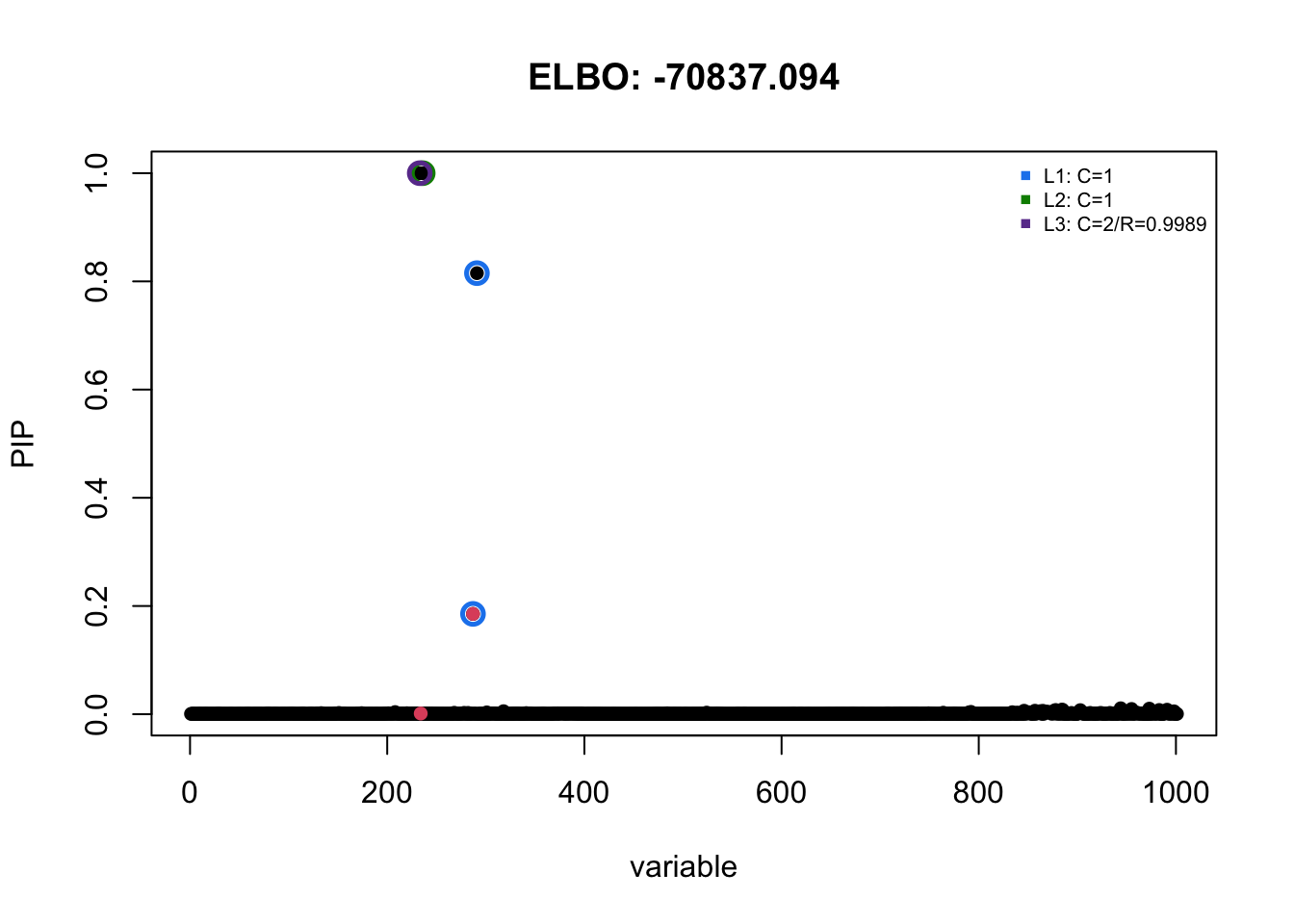

Past versions of unnamed-chunk-16-1.png

Version	Author	Date
5cea1d8	zouyuxin	2021-03-09
f4fd83c	zouyuxin	2021-03-06

Data 2

The region contains 1001 SNPs. There are three causals at 252, 340, 375.

d2 = dat$d2
b = d2$true_coef
idx = which(b!=0)

par(mfrow=c(1,2))
plot(d2$z, pch = 16, xlab = 'SNPs', ylab = 'z')
points(idx, d2$z[idx], col='red', pch = 16)
log10p = -log10(pnorm(-abs(d2$z))*2)
plot(log10p, pch = 16, xlab = 'SNPs', ylab = '-log10 p value')
points(idx, log10p[idx], col='red', pch = 16)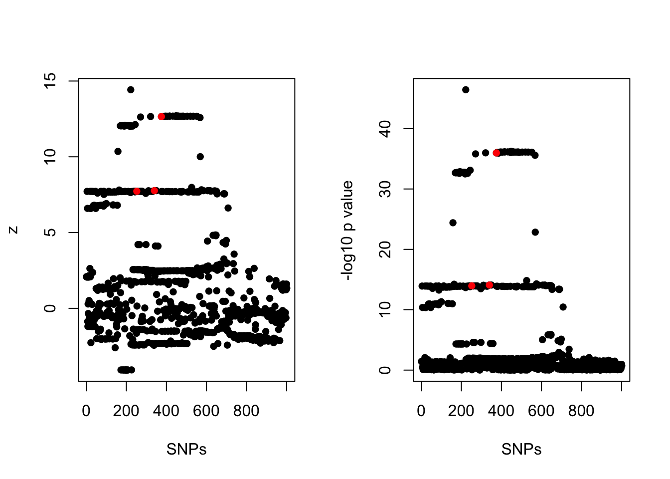

Past versions of unnamed-chunk-17-1.png

Version	Author	Date
5cea1d8	zouyuxin	2021-03-09
f4fd83c	zouyuxin	2021-03-06
065f6f7	zouyuxin	2021-03-06

The SNP with strongest marginal association is 222. The correlation between causal SNPs and top SNP is

cov2cor(d2$XtX)[c(222, idx), c(222, idx)]

              rs35291899_G rs2973016_A rs111613721_T rs145712863_T
rs35291899_G     1.0000000   0.5508992    0.55055773    0.79251604
rs2973016_A      0.5508992   1.0000000    0.99949772   -0.01428270
rs111613721_T    0.5505577   0.9994977    1.00000000   -0.01412418
rs145712863_T    0.7925160  -0.0142827   -0.01412418    1.00000000

Using L = 10, the susie model gives 1 CS.

f2 = susie_suff_stat(XtX = d2$XtX, Xty = d2$Xty, yty = d2$yty, n = d2$n, L=10, track_fit = T)
susie_plot(f2, y='PIP', b=b, add_legend = T, main=paste0('ELBO: ', round(susie_get_objective(f2), 4)))

Past versions of unnamed-chunk-19-1.png

Version	Author	Date
f4fd83c	zouyuxin	2021-03-06

It identifies the top SNP.

variable	1	2 (C)	3 (C)	4 (C)
SNP	222	252	340	375

susie_plot_iteration(f2, L=10, 'assets/susie_convergence_problem/susie_convergence_problem_d2_f3', pos=c(222, idx))

knitr::include_graphics("assets/susie_convergence_problem/susie_convergence_problem_d2_f3.gif", error = FALSE)

Past versions of susie_convergence_problem_d2_f3.gif

Version	Author	Date
f97ba78	zouyuxin	2021-03-06

Using L = 3, it converges to the same solution as L = 10.

f23 = susie_suff_stat(XtX = d2$XtX, Xty = d2$Xty, yty = d2$yty, n = d2$n, L=3, track_fit = T,
                     estimate_residual_variance = T, estimate_prior_variance = T)
susie_plot(f23, y='PIP', b=b, add_legend = T, main=paste0('ELBO: ', round(susie_get_objective(f23), 4)))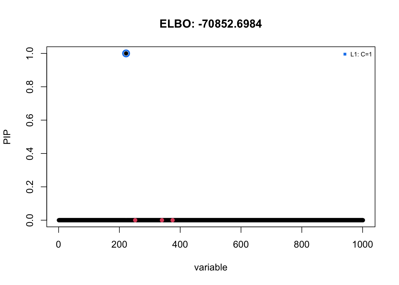

Past versions of unnamed-chunk-22-1.png

Version	Author	Date
5cea1d8	zouyuxin	2021-03-09
f4fd83c	zouyuxin	2021-03-06

We initialize at the truth,

beta_val = b[idx]
sinit = susieR::susie_init_coef(idx, beta_val, length(b))
f2true = susie_suff_stat(XtX = d2$XtX, Xty = d2$Xty, yty = d2$yty, n = d2$n, track_fit = T, s_init = sinit,
                            estimate_residual_variance = T,estimate_prior_variance = TRUE, max_iter = 200)
susie_plot(f2true, y='PIP', b=b, add_legend = T, main=paste0('ELBO: ', round(susie_get_objective(f2true), 4)))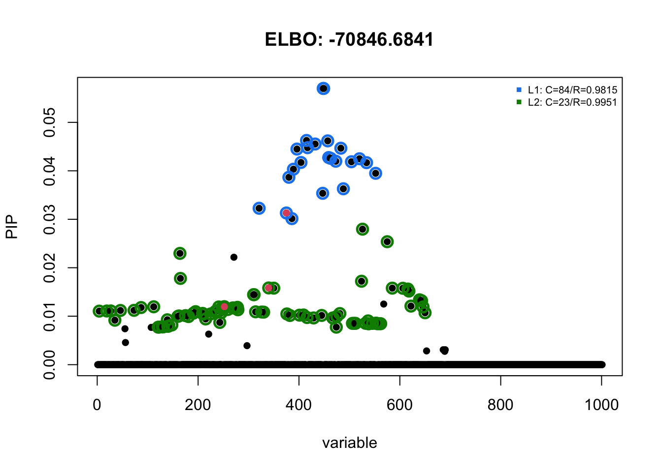

Past versions of unnamed-chunk-23-1.png

Version	Author	Date
5cea1d8	zouyuxin	2021-03-09

We try to initialize using LASSO solution:

fit.lasso = glmnet::glmnet(d2$X, d2$y, family="gaussian", alpha=1, dfmax = 10)
lasso.b = fit.lasso$beta[,max(which(fit.lasso$df <= 10))]
beta_idx = which(lasso.b != 0)
plot(fit.lasso, label=T)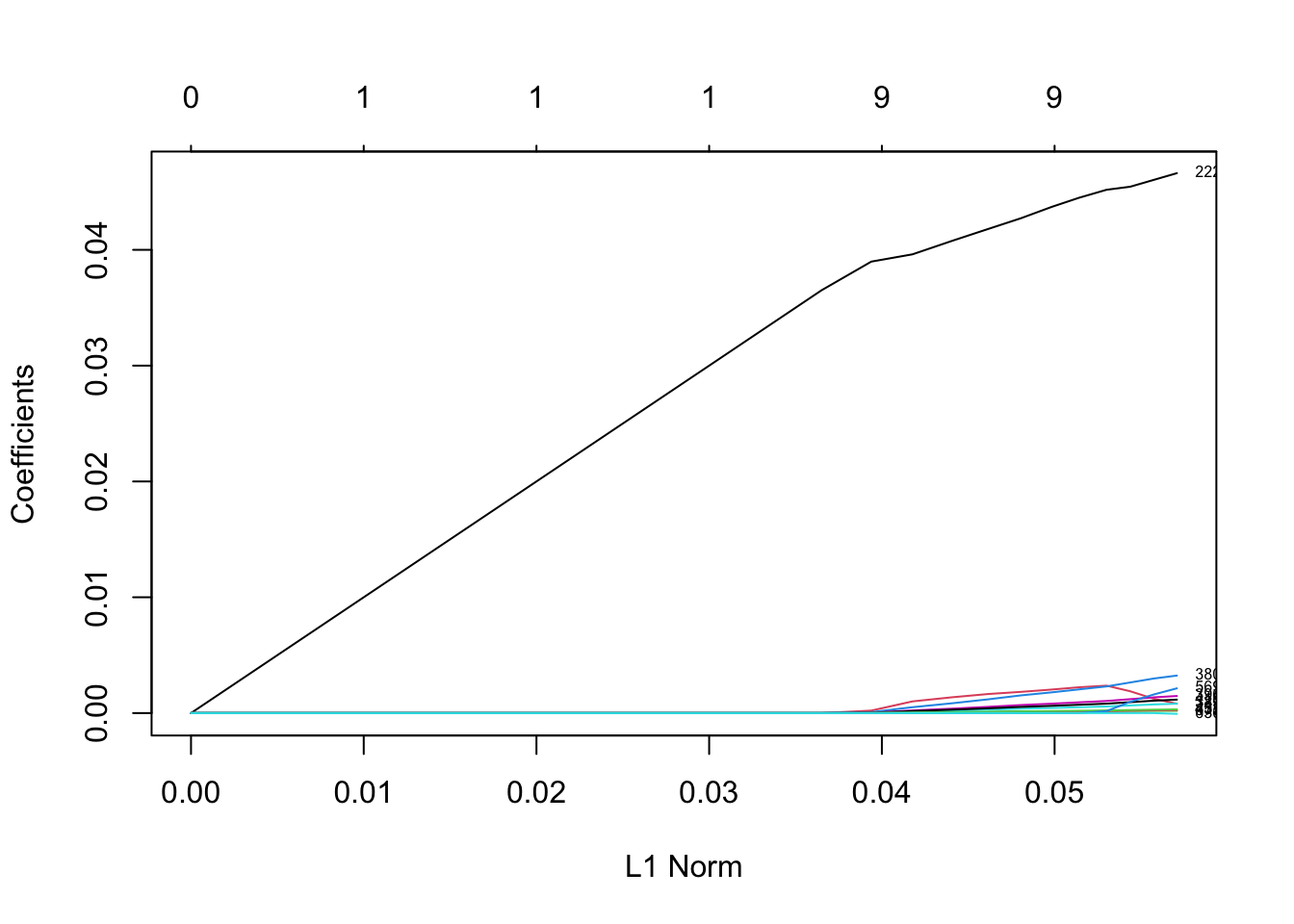

Past versions of unnamed-chunk-24-1.png

Version	Author	Date
5cea1d8	zouyuxin	2021-03-09

LASSO identifies one causal SNP 375 with non-zero effect. It also identifies SNP 222.

sinit = susieR::susie_init_coef(beta_idx, lasso.b[beta_idx], length(b))
f2lasso = susie_suff_stat(XtX = d2$XtX, Xty = d2$Xty, yty = d2$yty, n = d2$n, s_init = sinit,
                          estimate_residual_variance = T,estimate_prior_variance = TRUE,
                          max_iter = 200, track_fit = T)
susie_plot(f2lasso, y='PIP', b=b, add_legend = T, main=paste0('ELBO: ', round(susie_get_objective(f2lasso), 3)))

Past versions of unnamed-chunk-25-1.png

Version	Author	Date
5cea1d8	zouyuxin	2021-03-09

The priors for other CSs shrink to 0 at the first iteration.

susie_plot_iteration(f2lasso, L=nrow(resinit$alpha), 'assets/susie_convergence_problem/susie_convergence_problem_d2_finitlasso', pos=sort(c(beta_idx, idx)))

knitr::include_graphics("assets/susie_convergence_problem/susie_convergence_problem_d2_finitlasso.gif", error = FALSE)

Past versions of susie_convergence_problem_d2_finitlasso.gif

Version	Author	Date
afbca11	zouyuxin	2021-03-06

We try LASSO with CV:

fit.lassocv = glmnet::cv.glmnet(d2$X, d2$y, family="gaussian", alpha=1)
lassocv.b = as.vector(coef(fit.lassocv, s = "lambda.min"))[-1]
beta_idx <- sort(abs(lassocv.b), index.return=TRUE, decreasing=TRUE)$ix[1:10]

The LASSO solution does not contain any causal SNPs.

sinit = susieR::susie_init_coef(beta_idx, lassocv.b[beta_idx], length(b))
f2lassosv = susie_suff_stat(XtX = d2$XtX, Xty = d2$Xty, yty = d2$yty, n = d2$n, s_init = sinit,
                          estimate_residual_variance = T,estimate_prior_variance = TRUE,
                          max_iter = 200, track_fit = T)
susie_plot(f2lassosv, y='PIP', b=b, add_legend = T, main=paste0('ELBO: ', round(susie_get_objective(f2lassosv), 3)))

Past versions of unnamed-chunk-29-1.png

Version	Author	Date
5cea1d8	zouyuxin	2021-03-09

We try mr.ash initialize with LASSO cv solution.

library(mr.ash.alpha)
fmrash = mr.ash(d2$X, d2$y, beta.init = lassocv.b)

Mr.ASH terminated at iteration 18.

Mr.ash identifies SNP 222.

plot(fmrash$beta)
points(idx, fmrash$beta[idx], col='red', pch=16)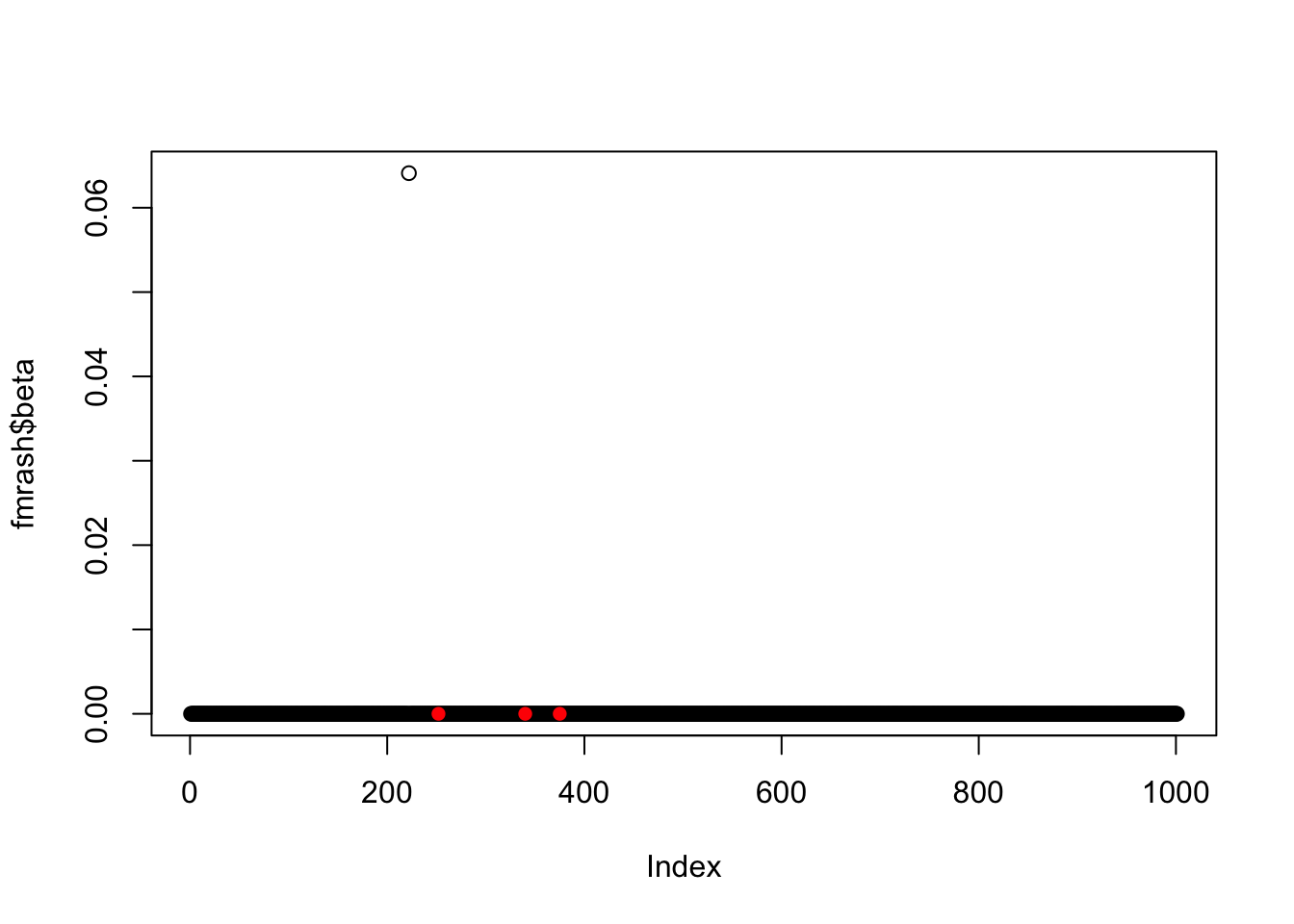

Past versions of unnamed-chunk-31-1.png

Version	Author	Date
5cea1d8	zouyuxin	2021-03-09

We try L0Learn.

set.seed(1)
L0fit = L0Learn.cvfit(d2$X, d2$y, penalty = "L0")
lambdaIndex = which.min(L0fit$cvMeans[[1]]) 
L0coef = as.numeric(coef(L0fit$fit, lambda = L0fit$fit$lambda[[1]][lambdaIndex]))
effect.beta = L0coef[which(L0coef!=0)][-1]
effect.index = (which(L0coef!=0)-1)[-1] 

The effect SNPs are

effect.index

[1] 169 222

s.init = susie_init_coef(effect.index, effect.beta, length(b))
f2L0.fit = susie_suff_stat(XtX = d2$XtX, Xty = d2$Xty, yty = d2$yty, n = d1$n, s_init = s.init,
                          estimate_residual_variance = T,estimate_prior_variance = TRUE,
                          max_iter = 200, track_fit = T)
susie_plot(f2L0.fit, y='PIP', b=b, add_legend = T, main=paste0('ELBO: ', round(susie_get_objective(f2L0.fit), 3)))

Past versions of unnamed-chunk-34-1.png

Version	Author	Date
5cea1d8	zouyuxin	2021-03-09

Data 3

The region contains 1001 SNPs. There are two causals at 435, 450. Default initialization works. LASSO initialization doesn’t work.

d3 = dat$d3
b = d3$true_coef
idx = which(b!=0)

par(mfrow=c(1,2))
plot(d3$z, pch = 16, xlab = 'SNPs', ylab = 'z')
points(idx, d3$z[idx], col='red', pch = 16)
log10p = -log10(pnorm(-abs(d3$z))*2)
plot(log10p, pch = 16, xlab = 'SNPs', ylab = '-log10 p value')
points(idx, log10p[idx], col='red', pch = 16)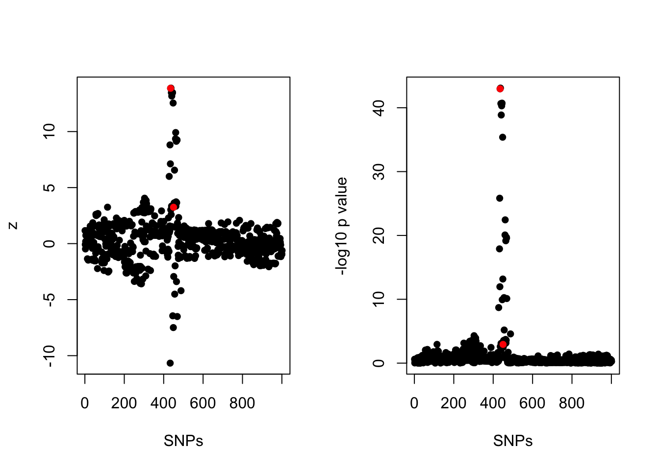

Past versions of unnamed-chunk-35-1.png

Version	Author	Date
5cea1d8	zouyuxin	2021-03-09

With default initialization:

f3 = susie_suff_stat(XtX = d3$XtX, Xty = d3$Xty, yty = d3$yty, n = d3$n, L=10, track_fit = T)
susie_plot(f3, y='PIP', b=b, add_legend = T, main=paste0('ELBO: ', round(susie_get_objective(f3), 4)))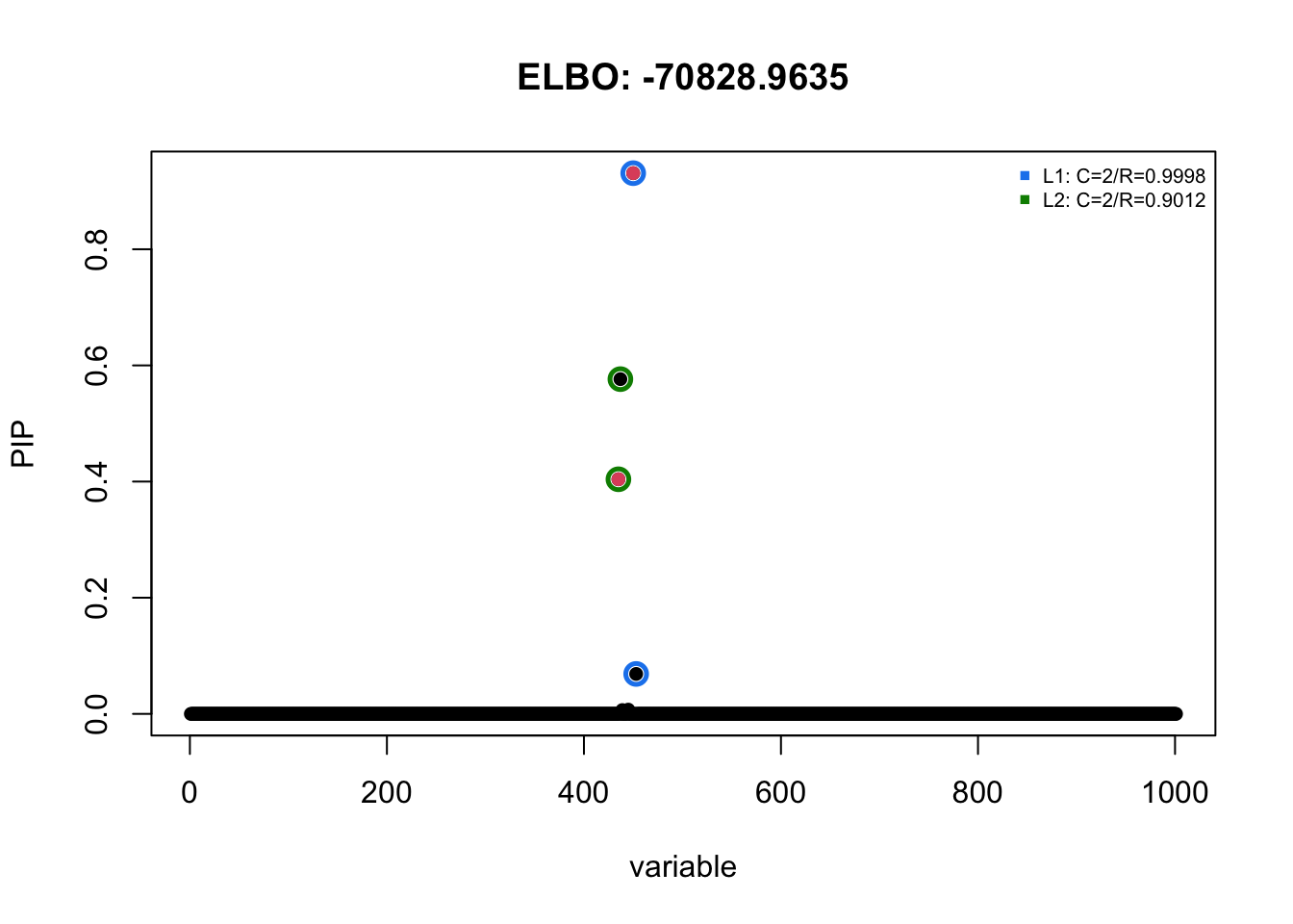

With LASSO with CV initialization:

fit.lassocv = glmnet::cv.glmnet(d3$X, d3$y, family="gaussian", alpha=1)
lassocv.b = as.vector(coef(fit.lassocv, s = "lambda.min"))[-1]
beta_idx <- sort(abs(lassocv.b), index.return=TRUE, decreasing=TRUE)$ix[1:10]
beta_idx = beta_idx[lassocv.b[beta_idx]!=0]

LASSO picks the following SNPs:

beta_idx

 [1] 435 448 443 437 433 463 333 843 457  40

sinit = susieR::susie_init_coef(beta_idx, lassocv.b[beta_idx], length(b))
f3lasso = susie_suff_stat(XtX = d3$XtX, Xty = d3$Xty, yty = d3$yty, n = d3$n, s_init = sinit,
                          estimate_residual_variance = T,estimate_prior_variance = TRUE,
                          max_iter = 200, track_fit = T)
susie_plot(f3lasso, y='PIP', b=b, add_legend = T, main=paste0('ELBO: ', round(susie_get_objective(f3lasso), 3)))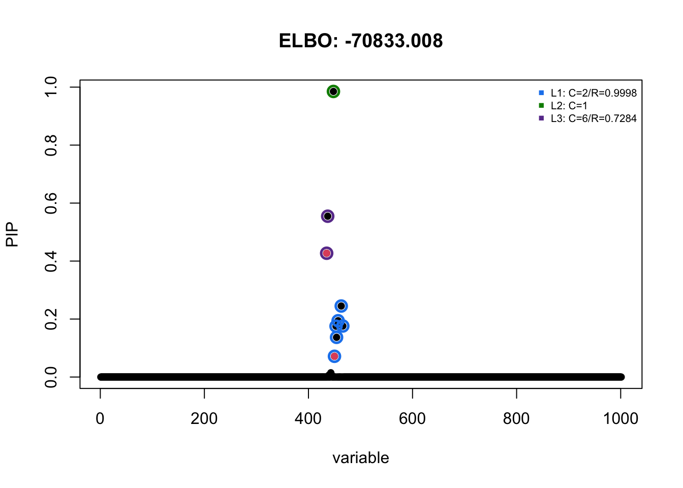

Session information

sessionInfo()

R version 4.0.3 (2020-10-10)
Platform: x86_64-apple-darwin17.0 (64-bit)
Running under: macOS Big Sur 10.16

Matrix products: default
BLAS:   /Library/Frameworks/R.framework/Versions/4.0/Resources/lib/libRblas.dylib
LAPACK: /Library/Frameworks/R.framework/Versions/4.0/Resources/lib/libRlapack.dylib

locale:
[1] en_US.UTF-8/en_US.UTF-8/en_US.UTF-8/C/en_US.UTF-8/en_US.UTF-8

attached base packages:
[1] stats     graphics  grDevices utils     datasets  methods   base     

other attached packages:
[1] mr.ash.alpha_0.1-36 L0Learn_2.0.0       susieR_0.10.0      
[4] workflowr_1.6.2    

loaded via a namespace (and not attached):
 [1] Rcpp_1.0.6       plyr_1.8.6       pillar_1.4.7     compiler_4.0.3  
 [5] later_1.1.0.1    git2r_0.27.1     iterators_1.0.13 tools_4.0.3     
 [9] digest_0.6.27    evaluate_0.14    lifecycle_1.0.0  tibble_3.0.6    
[13] gtable_0.3.0     lattice_0.20-41  pkgconfig_2.0.3  rlang_0.4.10    
[17] foreach_1.5.1    Matrix_1.2-18    yaml_2.2.1       xfun_0.19       
[21] stringr_1.4.0    dplyr_1.0.2      knitr_1.30       generics_0.1.0  
[25] fs_1.5.0         vctrs_0.3.6      glmnet_4.0-2     tidyselect_1.1.0
[29] rprojroot_2.0.2  grid_4.0.3       reshape_0.8.8    glue_1.4.2      
[33] R6_2.5.0         survival_3.2-7   rmarkdown_2.5    reshape2_1.4.4  
[37] purrr_0.3.4      ggplot2_3.3.3    magrittr_2.0.1   whisker_0.4     
[41] MASS_7.3-53      splines_4.0.3    codetools_0.2-18 scales_1.1.1    
[45] promises_1.1.1   ellipsis_0.3.1   htmltools_0.5.0  shape_1.4.5     
[49] colorspace_2.0-0 httpuv_1.5.4     stringi_1.5.3    munsell_0.5.0   
[53] crayon_1.4.1