estimation of effect sizes and detection of significant effects
Zhiwei Ma
2017
Last updated: 2017-10-08
Code version: c7a9038
Overview
In this files, we analyze the accuracy of estimaiton of effect sizes and the detection of significant effects. To measure the accuracy, we apply the relative root mean squrared error (RRMSE). An RRMSE < 1 indicates the methods produces estimates that are more accurate than the original obserbation \(\hat\beta\). For detection of significant effects, we require the estimated sign of each significant effect to be correct to be considered a “true positive”.
Results
Simulation 1
We set unit number \(n = 5000\), and study number \(R = 4\). We set every observation has the same standard error, \(s_{jr}=1\). That is \(\hat\beta_{jr}|\beta_{jr}\sim N(\beta_{jr};0,1)\). The 5000 units come from 4 patterns (\(K=4\)): 4500 units have zero effects in all four studies, that is \(\beta_{jr}=0\), for \(r = 1,2,3,4\); 200 units have effect \(\beta_{jr}\sim N(0,4^2)\) for \(r =1, 2\) and \(\beta_{jr}=0\) for \(r =3, 4\); 200 units have effect \(\beta_{jr}\sim N(0,4^2)\) for \(r =3, 4\) and \(\beta_{jr}=0\) for \(r = 1, 2\); 100 unitss have effect \(\beta_{jr}\sim N(0,4^2)\) for \(r =1, 2,3,4\).
To fit the model, set \(K = 1:10\).
source('../code/function.R')
K = 4
D = 4
G = 5000
sigma2 = c(16,16,16,16)
pi0 = c(0.02,0.04,0.04,0.9)
q0 = matrix(0,nrow=K,ncol=D)
q0[1,] = c(1,1,1,1)
q0[2,] = c(1,1,0,0)
q0[3,] = c(0,1,1,0)
q0[4,] = c(0,0,0,0)
X = matrix(0,nrow=G,ncol=D)
Y = matrix(0,nrow=G,ncol=D)
rows = rep(1:K,times=pi0*G)
A = q0[rows,]
set.seed(111)
for(g in 1:G){
  for(d in 1:D){
    if(A[g,d]==1){
      X[g,d] = rnorm(1,0,sqrt(sigma2[d]))
    } else{
      X[g,d] = 0
    }
  }
}
beta = X
sebetahat=matrix(1,nrow=G,ncol=D)
betahat=matrix(10,nrow=G,ncol=D)
for(g in 1:G){
  for(d in 1:D){
    betahat[g,d] = rnorm(1,beta[g,d],sebetahat[g,d])
  }
}

# fit the model
fit1 = generic.cormotif(betahat,sebetahat,K=1:10,mess=FALSE)
The RRMSE for K = 1:10 is
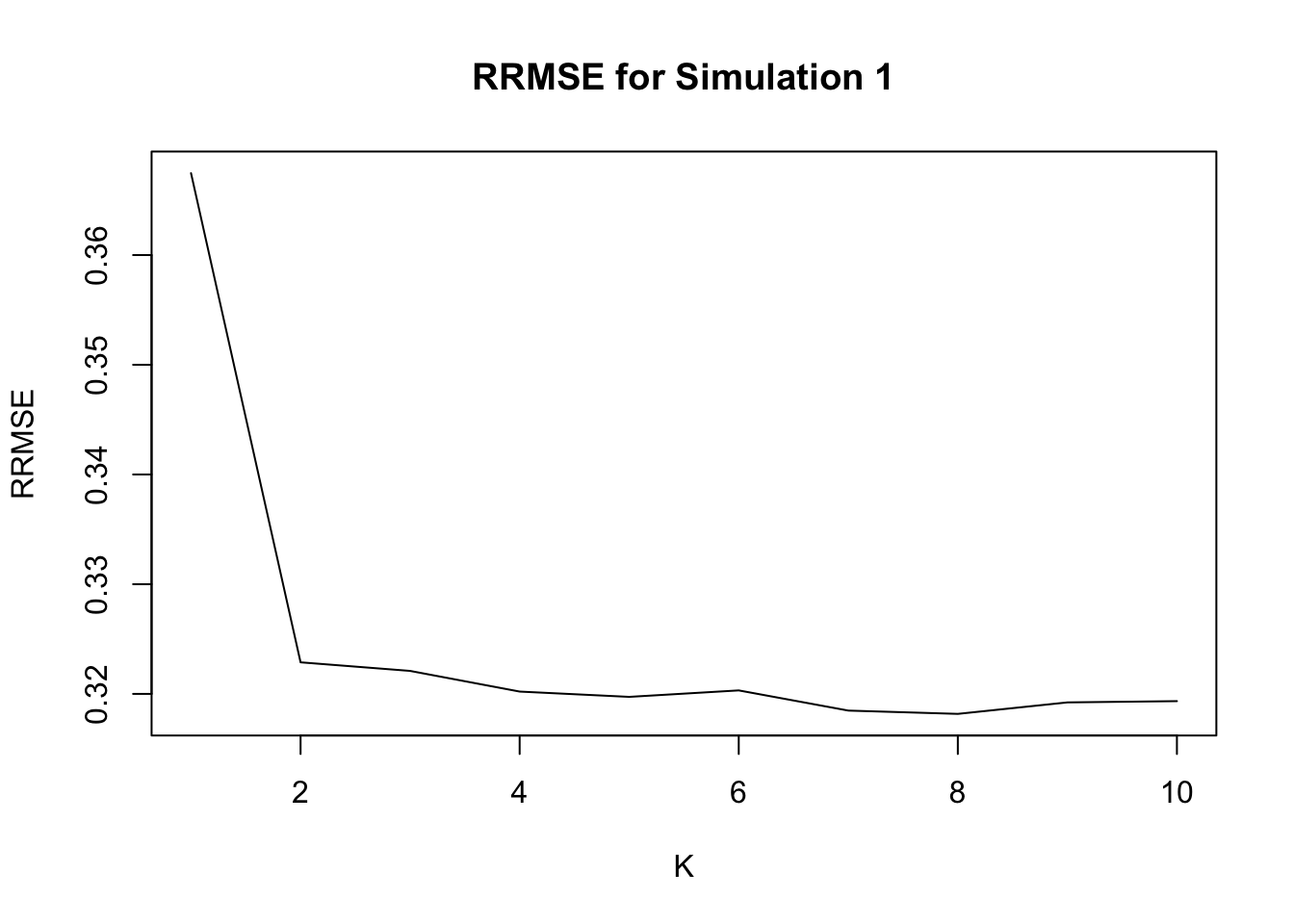
Notice that when \(K=1\), it is equvalent to applying ash to each study separately, and \(K = 4\) is the true model.
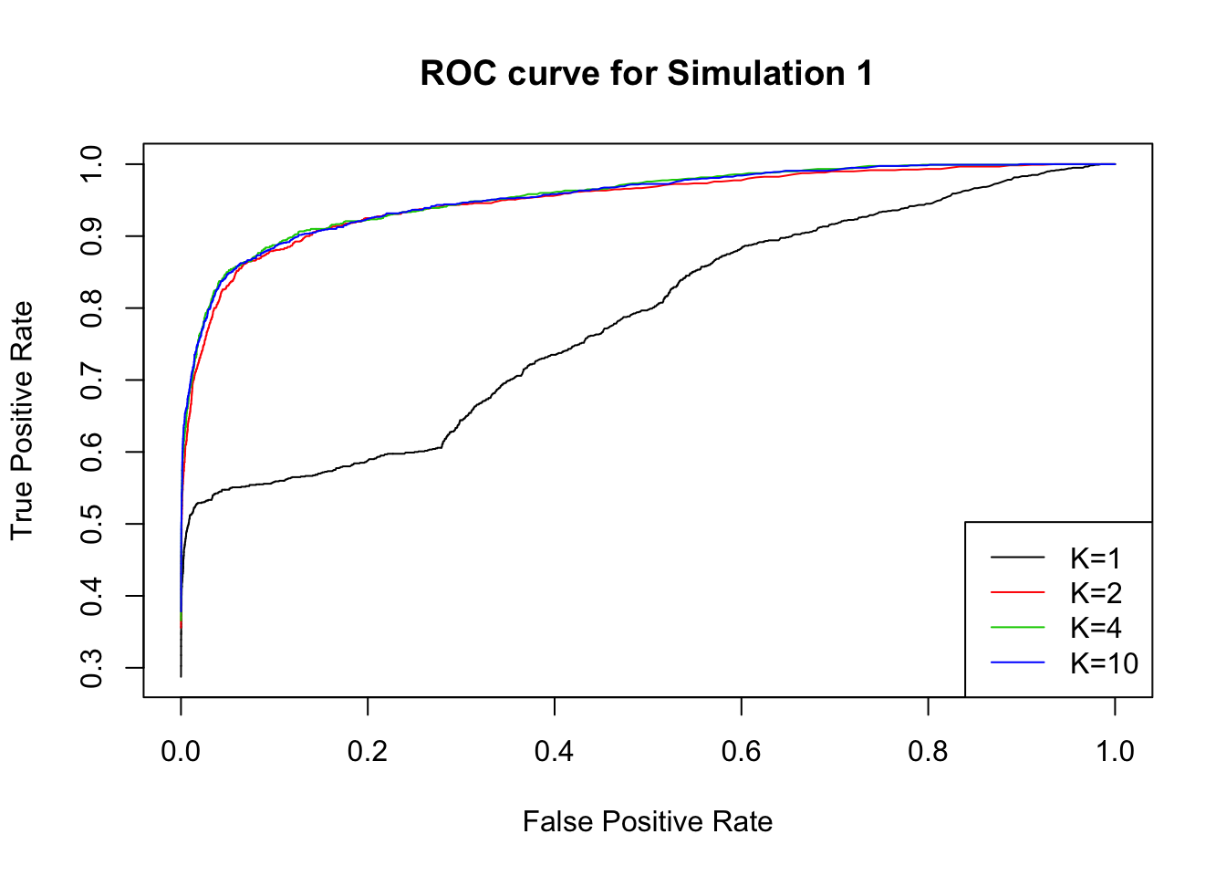
Changing the threshold for lfsr, we plot the ROC curve for \(K=1,2,4,10\).
Simulation 2
We set unit number \(n = 5000\), and study number \(R = 8\). We set every observation has the same standard error, \(s_{jr}=1\). That is \(\hat\beta_{jr}|\beta_{jr}\sim N(\beta_{jr};0,1)\). The 5000 units come from 5 patterns (\(K=5\)): 4000 units have zero effects in all four studies, that is \(\beta_{jr}=0\), for \(r = 1,2,3,4,5,6,7,8\); 250 units have effect \(\beta_{jr}\sim N(0,4^2)\) for \(r =1,2,3,4\) and \(\beta_{jr}=0\) for \(r =5, 6,7,8\); 250 units have effect \(\beta_{jr}\sim N(0,4^2)\) for \(r =5, 6,7,8\) and \(\beta_{jr}=0\) for \(r = 1,2,3,4\); 250 units have effect \(\beta_{jr}\sim N(0,4^2)\) for \(r =3,4,5,6\) and \(\beta_{jr}=0\) for \(r = 1,2,7,8\); 250 units have effect \(\beta_{jr}\sim N(0,4^2)\) for \(r =1,2,3,4,5,6,7,8\).
To fit the model, set \(K = 1:10\).
source('../code/function.R')
K = 5
D = 8
G = 5000
sigma2 = rep(16,D)
pi0 = c(0.05,0.05,0.05,0.05,0.8)
q0 = matrix(0,nrow=K,ncol=D)
q0[1,] = c(1,1,1,1,1,1,1,1)
q0[2,] = c(1,1,1,1,0,0,0,0)
q0[3,] = c(0,0,0,0,1,1,1,1)
q0[4,] = c(0,0,1,1,1,1,0,0)
q0[5,] = c(0,0,0,0,0,0,0,0)
X = matrix(0,nrow=G,ncol=D)
Y = matrix(0,nrow=G,ncol=D)
rows = rep(1:K,times=pi0*G)
A = q0[rows,]
set.seed(222)
for(g in 1:G){
  for(d in 1:D){
    if(A[g,d]==1){
      X[g,d] = rnorm(1,0,sqrt(sigma2[d]))
    } else{
      X[g,d] = 0
    }
  }
}
beta = X
sebetahat=matrix(1,nrow=G,ncol=D)
betahat=matrix(10,nrow=G,ncol=D)
for(g in 1:G){
  for(d in 1:D){
    betahat[g,d] = rnorm(1,beta[g,d],sebetahat[g,d])
  }
}
# fit the model
fit2 = generic.cormotif(betahat,sebetahat,K=1:10,mess=FALSE)
The RRMSE for K = 1:10 is
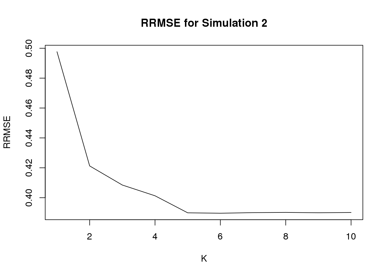
Notice that when \(K=1\), it is equvalent to applying ash to each study separately, and \(K=5\) is the true model.
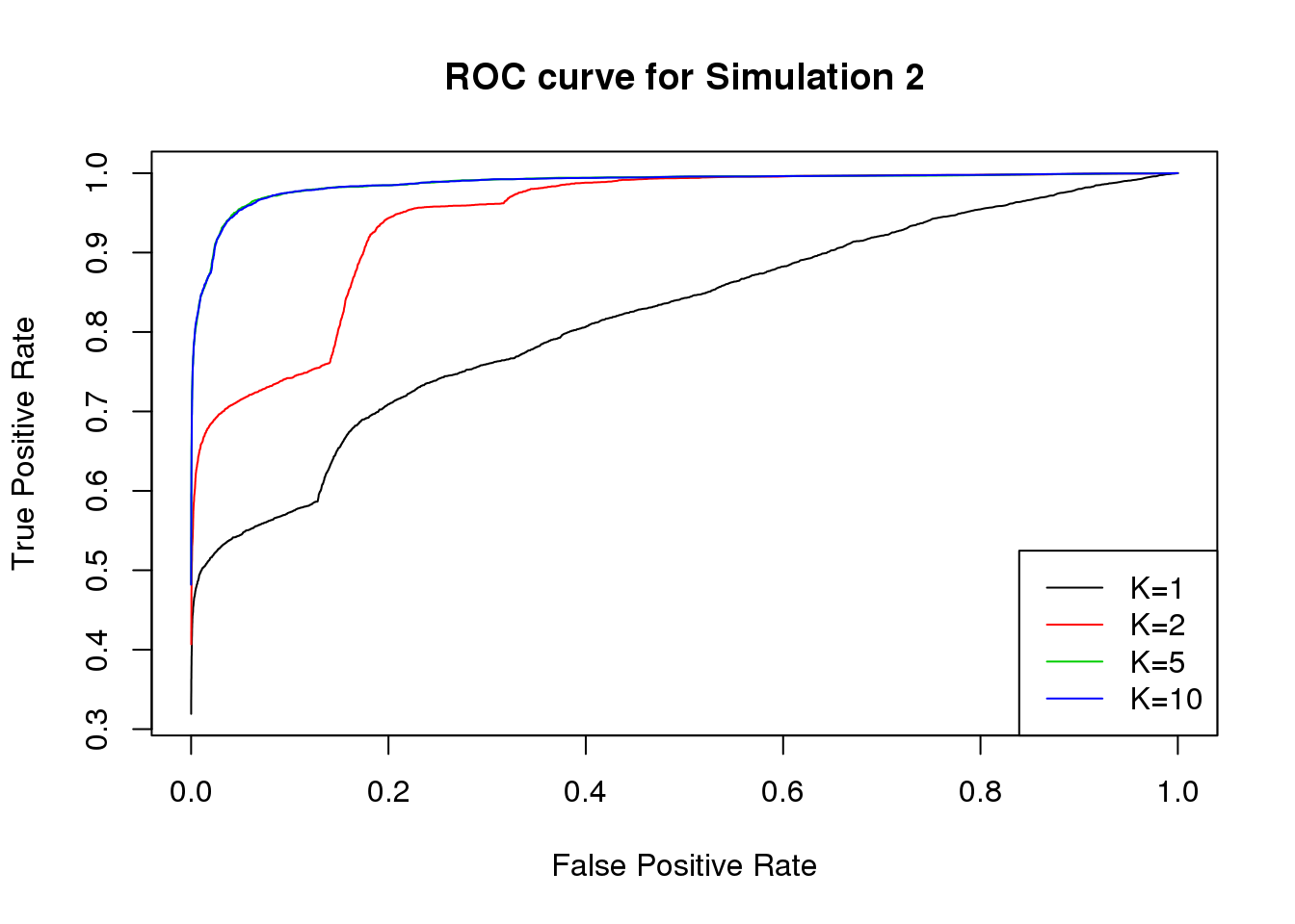
We plot the ROC curve for \(K=1,2,5,10\).
Session information
sessionInfo()R version 3.3.3 (2017-03-06)
Platform: x86_64-redhat-linux-gnu (64-bit)
Running under: Scientific Linux 7.2 (Nitrogen)
locale:
[1] LC_CTYPE=en_US.UTF-8 LC_NUMERIC=C
[3] LC_TIME=en_US.UTF-8 LC_COLLATE=en_US.UTF-8
[5] LC_MONETARY=en_US.UTF-8 LC_MESSAGES=en_US.UTF-8
[7] LC_PAPER=en_US.UTF-8 LC_NAME=C
[9] LC_ADDRESS=C LC_TELEPHONE=C
[11] LC_MEASUREMENT=en_US.UTF-8 LC_IDENTIFICATION=C
attached base packages:
[1] stats graphics grDevices utils datasets base
other attached packages:
[1] SQUAREM_2016.8-2
loaded via a namespace (and not attached):
[1] Rcpp_0.12.12 codetools_0.2-15 lattice_0.20-34
[4] digest_0.6.12 rprojroot_1.2 MASS_7.3-45
[7] grid_3.3.3 MatrixModels_0.4-1 backports_1.1.1
[10] git2r_0.19.0 magrittr_1.5 evaluate_0.10.1
[13] coda_0.19-1 stringi_1.1.5 SparseM_1.77
[16] Matrix_1.2-8 rmarkdown_1.6 tools_3.3.3
[19] stringr_1.2.0 compiler_3.3.3 yaml_2.1.14
[22] mcmc_0.9-5 htmltools_0.3.6 knitr_1.17
[25] quantreg_5.33 MCMCpack_1.4-0 methods_3.3.3 This R Markdown site was created with workflowr