Trend of Loglike

Last updated: 2017-10-03

Code version: 8300c85

Simulation 1

We set unit number \(n = 5000\), and study number \(R = 4\). We set every observation has the same standard error, \(s_{jr}=1\). That is \(\hat\beta_{jr}|\beta_{jr}\sim N(\beta_{jr};0,1)\). The 5000 units come from 4 patterns (\(K=4\)): 2500 units have zero effects in all four studies, that is \(\beta_{jr}=0\), for \(r = 1,2,3,4\); 1000 units have effect \(\beta_{jr}\sim N(0,4^2)\) for \(r =1, 2\) and \(\beta_{jr}=0\) for \(r =3, 4\); 1000 units have effect \(\beta_{jr}\sim N(0,4^2)\) for \(r =3, 4\) and \(\beta_{jr}=0\) for \(r = 1, 2\); 500 unitss have effect \(\beta_{jr}\sim N(0,4^2)\) for \(r =1, 2,3,4\).

To fit the model, set \(K = 1:10\).

source('../code/function.R')

# Simulate data
K = 4
D = 4
G = 5000
sigma2 = c(16,16,16,16)
pi0 = c(0.1,0.2,0.2,0.5)
q0 = matrix(0,nrow=K,ncol=D)
q0[1,] = c(1,1,1,1)
q0[2,] = c(1,1,0,0)
q0[3,] = c(0,0,1,1)
q0[4,] = c(0,0,0,0)
X = matrix(0,nrow=G,ncol=D)
rows = rep(1:K,times=pi0*G)
A = q0[rows,]
set.seed(222)
for(g in 1:G){
  for(d in 1:D){
    if(A[g,d]==1){
      X[g,d] = rnorm(1,0,sqrt(1+sigma2[d]))
    } else{
      X[g,d] = rnorm(1,0,1)
    }
  }
}
betahat=X
sebetahat=matrix(1,nrow=G,ncol=D)

#fit the model
fit1 = generic.cormotif(betahat,sebetahat,K=1:10,mess=FALSE)

The estimated \(\pi\) for \(K=4\)

fit1$allmotif[[4]]$pi

[1] 0.5152307 0.1937429 0.1002660 0.1907604

The estimated \(\pi\) for \(K=1：10\)

fit1$allmotif[[1]]$pi

[1] 1

fit1$allmotif[[2]]$pi

[1] 0.4644908 0.5355092

fit1$allmotif[[3]]$pi

[1] 0.5224704 0.2198905 0.2576391

fit1$allmotif[[4]]$pi

[1] 0.5152307 0.1937429 0.1002660 0.1907604

fit1$allmotif[[5]]$pi

[1] 0.50620682 0.02285662 0.18115366 0.19017075 0.09961214

fit1$allmotif[[6]]$pi

[1] 5.086825e-01 2.164448e-06 1.900644e-01 1.001864e-01 1.877408e-01
[6] 1.332366e-02

fit1$allmotif[[7]]$pi

[1] 0.503318240 0.004612764 0.009515062 0.102276967 0.185844317 0.191717590
[7] 0.002715060

fit1$allmotif[[8]]$pi

[1] 0.422545140 0.175224142 0.010880725 0.180928014 0.017286295 0.088767815
[7] 0.001773712 0.102594157

fit1$allmotif[[9]]$pi

[1] 0.488839540 0.181996345 0.017672553 0.166967541 0.008072951 0.008005716
[7] 0.087462374 0.037154767 0.003828213

fit1$allmotif[[10]]$pi

 [1] 4.169634e-01 8.993787e-03 8.218794e-04 1.031644e-08 9.905857e-02
 [6] 1.803221e-01 5.577992e-02 1.093727e-07 1.833917e-01 5.466845e-02

we can check the BIC and AIC values obtained by all cluster numbers:

plot(fit1$bic,type = "l",xlab = "K",ylab = "BIC")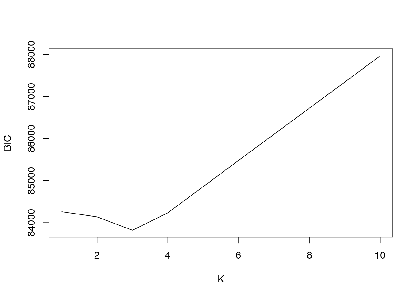

The AIC values:

plot(fit1$aic,type = "l",xlab = "K",ylab = "AIC")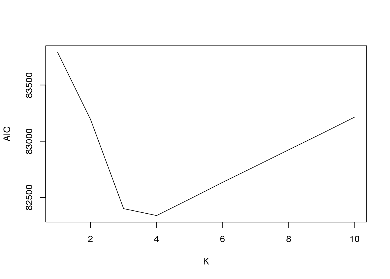

The loglikelihood values:

fit1$loglike

       K   loglike
 [1,]  1 -41823.66
 [2,]  2 -41451.30
 [3,]  3 -40982.05
 [4,]  4 -40878.30
 [5,]  5 -40878.55
 [6,]  6 -40880.08
 [7,]  7 -40879.18
 [8,]  8 -40878.86
 [9,]  9 -40877.94
[10,] 10 -40878.46

And plot

plot(fit1$loglike[,2],type = "l",xlab = "K",ylab = "loglike")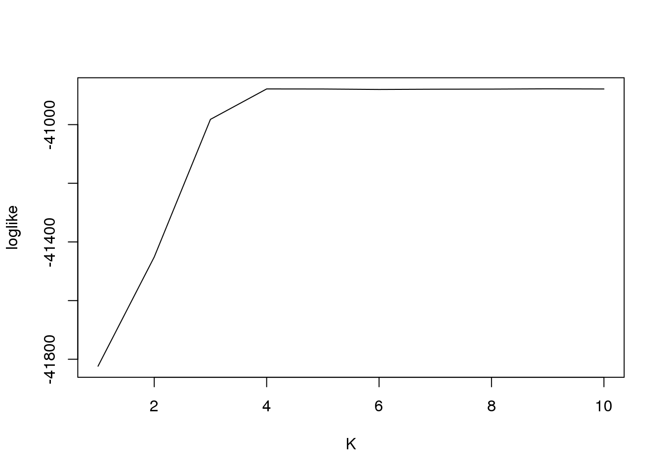

Simulation 2

With the same setting as simulation 1, just change \(\beta_{jr}\sim N(0,10^2)\), we check the same process.

To fit the model, set \(K = 1:10\).

source('../code/function.R')
# Simulate data
K = 4
D = 4
G = 5000
sigma2 = c(100,100,100,100)
pi0 = c(0.1,0.2,0.2,0.5)
q0 = matrix(0,nrow=K,ncol=D)
q0[1,] = c(1,1,1,1)
q0[2,] = c(1,1,0,0)
q0[3,] = c(0,0,1,1)
q0[4,] = c(0,0,0,0)
X = matrix(0,nrow=G,ncol=D)
rows = rep(1:K,times=pi0*G)
A = q0[rows,]
set.seed(22)
for(g in 1:G){
  for(d in 1:D){
    if(A[g,d]==1){
      X[g,d] = rnorm(1,0,sqrt(1+sigma2[d]))
    } else{
      X[g,d] = rnorm(1,0,1)
    }
  }
}
betahat=X
sebetahat=matrix(1,nrow=G,ncol=D)
#fit the model
fit2 = generic.cormotif(betahat,sebetahat,K=1:10,mess=FALSE)

The estimated \(\pi\) for \(K=4\)

fit2$allmotif[[4]]$pi

[1] 0.49808427 0.20541469 0.09356433 0.20293671

The estimated \(\pi\) for \(K=1：10\)

fit2$allmotif[[1]]$pi

[1] 1

fit2$allmotif[[2]]$pi

[1] 0.4660542 0.5339458

fit2$allmotif[[3]]$pi

[1] 0.5136548 0.2710054 0.2153398

fit2$allmotif[[4]]$pi

[1] 0.49808427 0.20541469 0.09356433 0.20293671

fit2$allmotif[[5]]$pi

[1] 0.498721230 0.201836669 0.200606201 0.097336021 0.001499879

fit2$allmotif[[6]]$pi

[1] 0.500840921 0.034167764 0.063472418 0.199777532 0.200327966 0.001413399

fit2$allmotif[[7]]$pi

[1] 0.49732885 0.01521967 0.14690947 0.03524265 0.09087781 0.15302393
[7] 0.06139762

fit2$allmotif[[8]]$pi

[1] 0.430309620 0.001561974 0.165742957 0.069380330 0.096409887 0.034659757
[7] 0.164770406 0.037165068

fit2$allmotif[[9]]$pi

[1] 4.965642e-01 1.435156e-02 1.006954e-01 1.785711e-07 1.987861e-01
[6] 2.785602e-02 1.128664e-02 2.012593e-03 1.484473e-01

fit2$allmotif[[10]]$pi

 [1] 4.984091e-01 2.829495e-06 2.456831e-07 5.783959e-02 1.444550e-01
 [6] 7.416195e-02 3.760942e-06 2.616600e-06 2.331332e-02 2.018116e-01

we can check the BIC and AIC values obtained by all cluster numbers:

plot(fit2$bic,type = "l",xlab = "K",ylab = "BIC")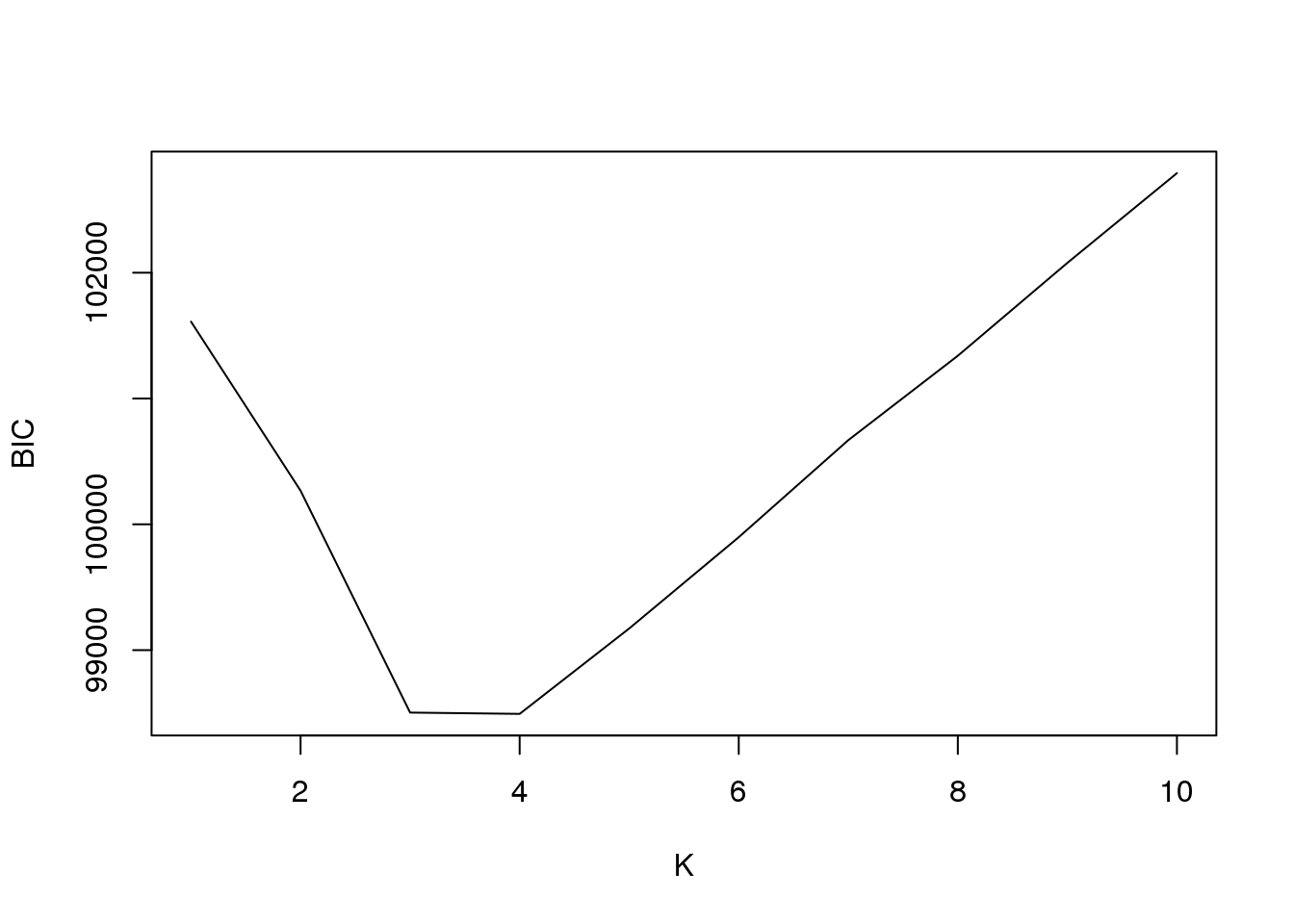

The AIC values:

plot(fit2$aic,type = "l",xlab = "K",ylab = "AIC")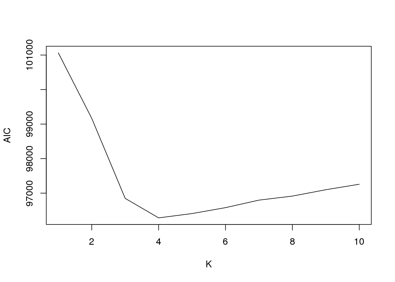

The loglikelihood values:

fit2$loglike

       K   loglike
 [1,]  1 -50447.73
 [2,]  2 -49413.89
 [3,]  3 -48170.09
 [4,]  4 -47802.94
 [5,]  5 -47780.43
 [6,]  6 -47781.19
 [7,]  7 -47804.89
 [8,]  8 -47778.40
 [9,]  9 -47785.58
[10,] 10 -47780.08

And plot

plot(fit2$loglike[,2],type = "l",xlab = "K",ylab = "loglike")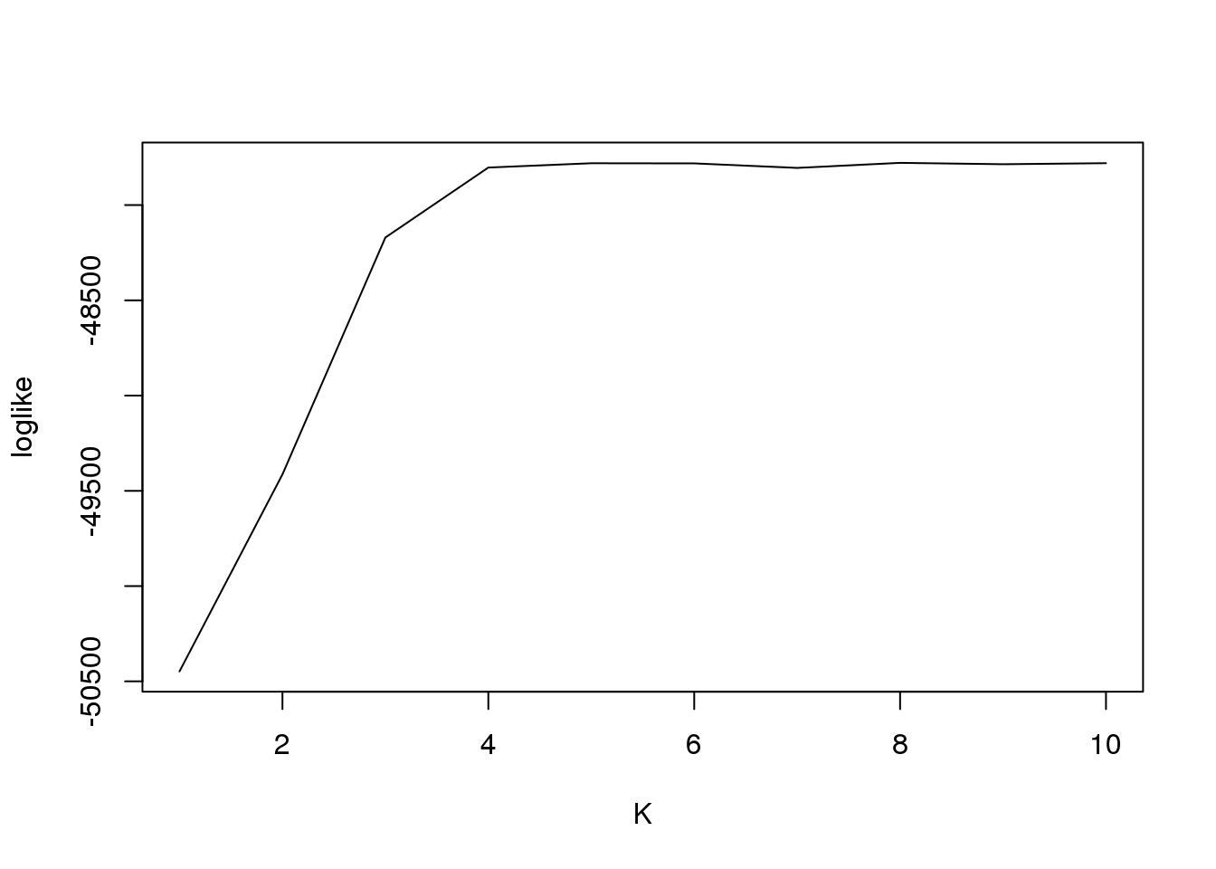

Simulation 3

With the same setting as simulation 1, just change the proportion of 4 patterns to 1250:1250:1250:1250, we check the same process.

To fit the model, set \(K = 1:10\).

source('../code/function.R')
# Simulate data
K = 4
D = 4
G = 5000
sigma2 = c(16,16,16,16)
pi0 = c(0.25,0.25,0.25,0.25)
q0 = matrix(0,nrow=K,ncol=D)
q0[1,] = c(1,1,1,1)
q0[2,] = c(1,1,0,0)
q0[3,] = c(0,0,1,1)
q0[4,] = c(0,0,0,0)
X = matrix(0,nrow=G,ncol=D)
rows = rep(1:K,times=pi0*G)
A = q0[rows,]
set.seed(333)
for(g in 1:G){
  for(d in 1:D){
    if(A[g,d]==1){
      X[g,d] = rnorm(1,0,sqrt(1+sigma2[d]))
    } else{
      X[g,d] = rnorm(1,0,1)
    }
  }
}
betahat=X
sebetahat=matrix(1,nrow=G,ncol=D)

#fit the model
fit3 = generic.cormotif(betahat,sebetahat,K=1:10,mess=FALSE)

The estimated \(\pi\) for \(K=4\)

fit3$allmotif[[4]]$pi

[1] 0.2608151 0.2594400 0.2648796 0.2148653

The estimated \(\pi\) for \(K=1：10\)

fit3$allmotif[[1]]$pi

[1] 1

fit3$allmotif[[2]]$pi

[1] 0.2440675 0.7559325

fit3$allmotif[[3]]$pi

[1] 0.2969971 0.4100248 0.2929781

fit3$allmotif[[4]]$pi

[1] 0.2608151 0.2594400 0.2648796 0.2148653

fit3$allmotif[[5]]$pi

[1] 0.25889418 0.18572877 0.25629099 0.25298173 0.04610434

fit3$allmotif[[6]]$pi

[1] 0.26335597 0.18971267 0.05430347 0.06806653 0.21531393 0.20924742

fit3$allmotif[[7]]$pi

[1] 2.683070e-01 2.623840e-01 5.887496e-03 2.148667e-01 2.669345e-02
[6] 7.051387e-07 2.218608e-01

fit3$allmotif[[8]]$pi

[1] 2.724083e-01 1.873649e-01 2.393964e-01 6.686674e-06 2.253818e-01
[6] 1.922407e-02 3.596410e-02 2.025374e-02

fit3$allmotif[[9]]$pi

[1] 0.25676523 0.02451442 0.25365626 0.17996013 0.01476107 0.02243582
[7] 0.00545013 0.17506744 0.06738950

fit3$allmotif[[10]]$pi

 [1] 2.630456e-01 2.373367e-02 8.543618e-03 6.207178e-02 2.623374e-07
 [6] 2.164205e-01 1.234637e-07 2.514193e-01 2.562691e-07 1.747649e-01

we can check the BIC and AIC values obtained by all cluster numbers:

plot(fit3$bic,type = "l",xlab = "K",ylab = "BIC")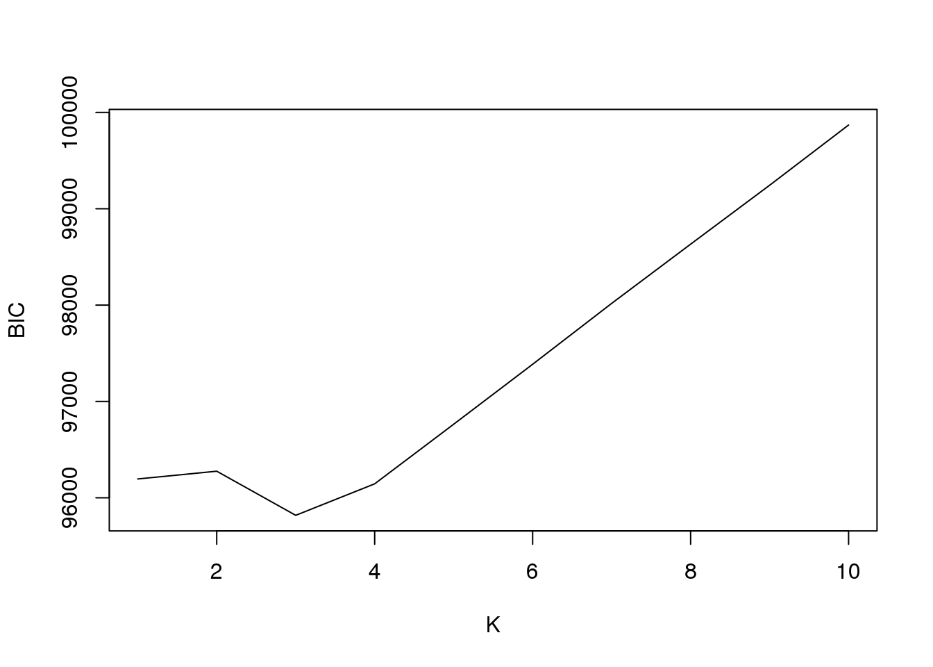

The AIC values:

plot(fit3$aic,type = "l",xlab = "K",ylab = "AIC")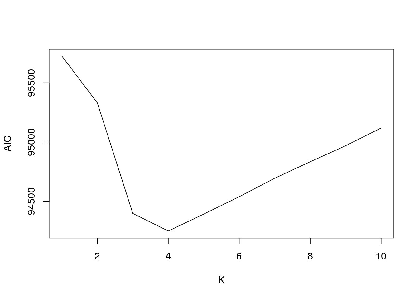

The loglikelihood values:

fit3$loglike

       K   loglike
 [1,]  1 -47791.09
 [2,]  2 -47520.42
 [3,]  3 -46980.58
 [4,]  4 -46833.20
 [5,]  5 -46831.61
 [6,]  6 -46832.02
 [7,]  7 -46836.93
 [8,]  8 -46833.53
 [9,]  9 -46828.33
[10,] 10 -46830.18

And plot

plot(fit3$loglike[,2],type = "l",xlab = "K",ylab = "loglike")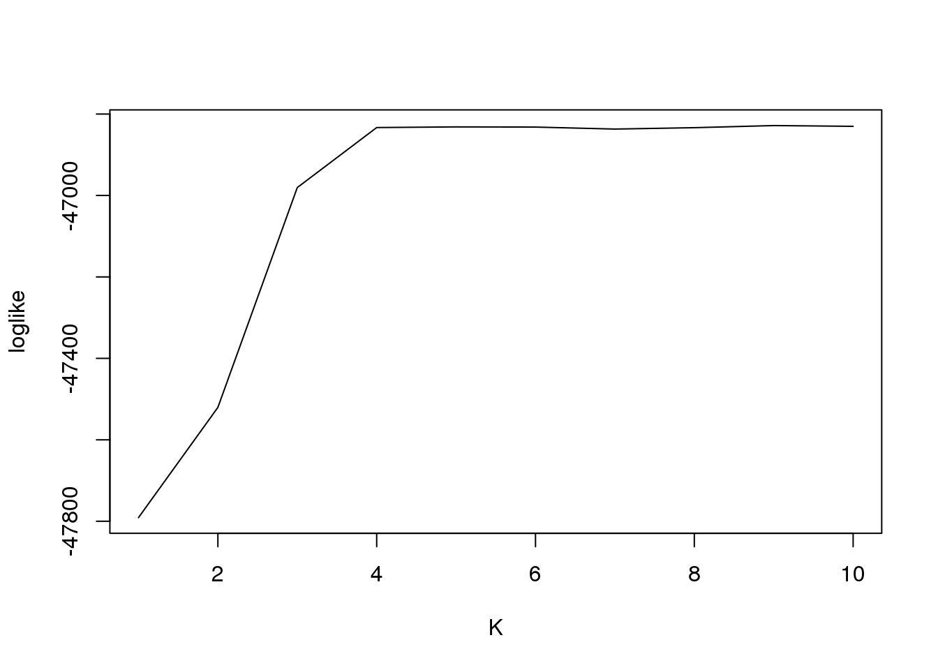

Session information

sessionInfo()

R version 3.3.3 (2017-03-06)
Platform: x86_64-redhat-linux-gnu (64-bit)
Running under: Scientific Linux 7.2 (Nitrogen)

locale:
 [1] LC_CTYPE=en_US.UTF-8       LC_NUMERIC=C              
 [3] LC_TIME=en_US.UTF-8        LC_COLLATE=en_US.UTF-8    
 [5] LC_MONETARY=en_US.UTF-8    LC_MESSAGES=en_US.UTF-8   
 [7] LC_PAPER=en_US.UTF-8       LC_NAME=C                 
 [9] LC_ADDRESS=C               LC_TELEPHONE=C            
[11] LC_MEASUREMENT=en_US.UTF-8 LC_IDENTIFICATION=C       

attached base packages:
[1] stats     graphics  grDevices utils     datasets  base     

other attached packages:
[1] SQUAREM_2016.8-2

loaded via a namespace (and not attached):
 [1] Rcpp_0.12.12       codetools_0.2-15   lattice_0.20-34   
 [4] digest_0.6.12      rprojroot_1.2      MASS_7.3-45       
 [7] grid_3.3.3         MatrixModels_0.4-1 backports_1.1.1   
[10] git2r_0.19.0       magrittr_1.5       evaluate_0.10.1   
[13] coda_0.19-1        stringi_1.1.5      SparseM_1.77      
[16] Matrix_1.2-8       rmarkdown_1.6      tools_3.3.3       
[19] stringr_1.2.0      compiler_3.3.3     yaml_2.1.14       
[22] mcmc_0.9-5         htmltools_0.3.6    knitr_1.17        
[25] quantreg_5.33      MCMCpack_1.4-0     methods_3.3.3

This R Markdown site was created with workflowr

Trend of Loglike

Zhiwei Ma

9/24/2017

Simulation 1

Simulation 2

Simulation 3

Session information