Simulation for Correlation Motif
Zhiwei Ma
8/30/2017
Last updated: 2017-09-15
Code version: e7afefa
Model Framework
The framework of Correlation Motif model is based on my write-up document and supplementary matrials by \(Wei\) \(and\) \(Ji\) (2015). In \(Wei\) \(and\) \(Ji\) (2015), they implemented an EM algorithm and introduced priors for both \(\pi\) and \(Q\). As a result, their iterative formulas for new \(\pi\) and new \(Q\) are:
\[\begin{eqnarray} \pi_k^{(t+1)} = \frac{\sum_{i=1}^n p_{ik}+1}{n+K} , \\ q_{kr}^ {(t+1)}=\frac{\sum_{i=1}^n p_{ikr1}+1}{\sum_{i=1}^n p_{ik}+2}. \end{eqnarray}\]However, one can apply EM algorithm without introducing a prior and obtain a more interpretable formula:
\[\begin{eqnarray} \pi_k^{(t+1)} = \frac{1}{n} \sum_{i=1}^n p_{ik}, \\ q_{kr}^ {(t+1)}=\frac{\sum_{i=1}^n p_{ikr1}}{\sum_{i=1}^n p_{ik}}. \end{eqnarray}\]Here \(p_{ik}= Pr(z_i=k|X_i,\pi^{(t)}, Q^ {(t)})\) is the posterior probability for gene \(i\) belonging to class \(k\), and the mean of \(p_{ik}\) over \(i\) is a reasonable estimations for \(\pi_{k}\). The argument is similar for \(q_{kr}\). Thus, we could interpret the underlying meaning in our iterative formulas.
In fact, since \(G\) is relatively large and \(G \gg K\), the two formulas tend to give very similar results. We will illustrate this idea by implementing these two algorithms seperately on the same dataset: \(simudata2\) in R package \(Cormotif\).
Notice that right now we are using the model applying limma (\(Smyth\), 2004). The results with prior is
library(Cormotif)
data(simudata2)
exprs.simu2<-as.matrix(simudata2[,2:25])
data(simu2_groupid)
data(simu2_compgroup)

motif.fitted<-cormotiffit(exprs.simu2,simu2_groupid,simu2_compgroup,
                          K=1:5,max.iter=1000,BIC=TRUE)
[1] "We have run the first 50 iterations for K=3"
[1] "We have run the first 100 iterations for K=3"
[1] "We have run the first 50 iterations for K=4"
[1] "We have run the first 100 iterations for K=4"
[1] "We have run the first 150 iterations for K=4"
[1] "We have run the first 200 iterations for K=4"
[1] "We have run the first 250 iterations for K=4"
[1] "We have run the first 300 iterations for K=4"
[1] "We have run the first 350 iterations for K=4"
[1] "We have run the first 400 iterations for K=4"
[1] "We have run the first 450 iterations for K=4"
[1] "We have run the first 50 iterations for K=5"
[1] "We have run the first 100 iterations for K=5"
[1] "We have run the first 150 iterations for K=5"
[1] "We have run the first 200 iterations for K=5"
[1] "We have run the first 250 iterations for K=5"motif.fitted$bic K bic
[1,] 1 44688.73
[2,] 2 44235.64
[3,] 3 44210.76
[4,] 4 44227.07
[5,] 5 44247.30plotIC(motif.fitted)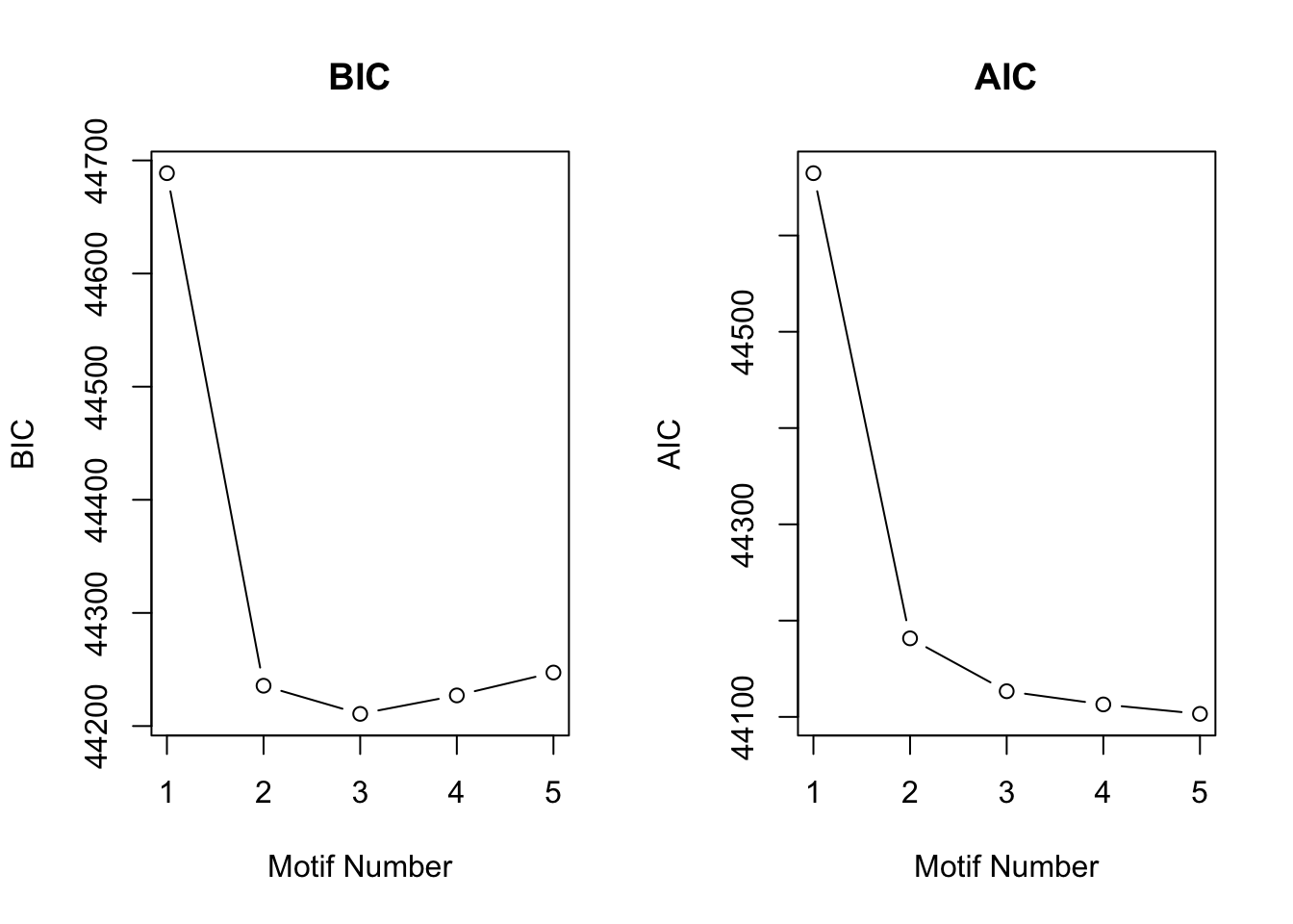
plotMotif(motif.fitted)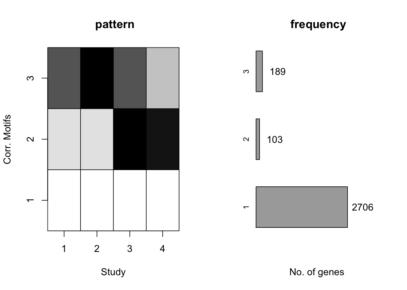
The results without prior is
motif.fitted<-cormotiffit_1(exprs.simu2,simu2_groupid,simu2_compgroup,K=1:5,max.iter=1000,BIC=TRUE)

motif.fitted$bic
K bic
[1,] 1 44688.71
[2,] 2 44232.37
[3,] 3 44202.89
[4,] 4 44218.54
[5,] 5 44234.69plotIC(motif.fitted)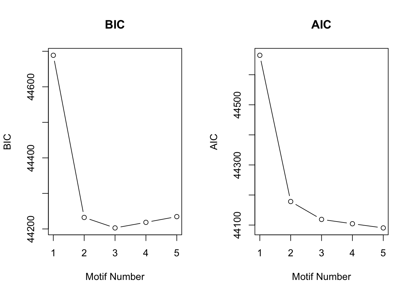
plotMotif(motif.fitted)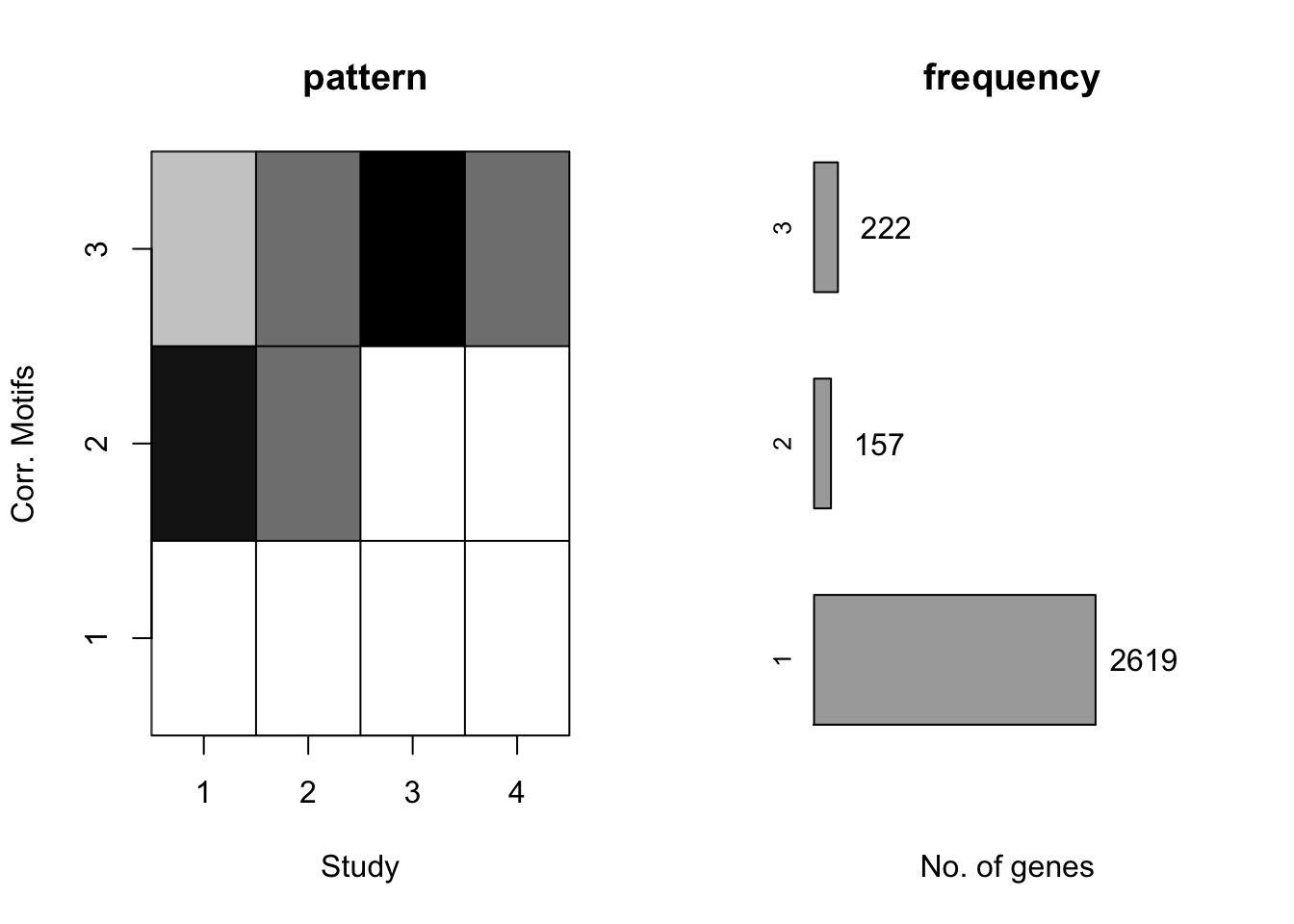
The two methods do give very similar results. However in practice, it takes much less iterations for methods with prior to achieve its accuracy. Here we prefer to apply CorMotif with prior. In the rest of document, without specification, we apply CorMOtif with prior.
Simulation based on limma
We first duplicated several simulation from \(Wei\) \(and\) \(Ji\) (2015), which was still based on limma.
Simulation 1
In simulation 1, we generated 10,000 genes and four studies according to the four different patterns: 100 genes were differentially expressed in all four studies (\(Y_i = [1,1,1,1]\)); 400 genes were differential only in studies 1 and 2 (\(Y_i = [1,1,0,0]\)); 400 genes were differential only in studies 2 and 3 (\(Y_i = [0,1,1,0]\)); 9100 genes were non-differential (\(Y_i = [0,0,0,0]\)). Each study had six samples: three cases and three controls. The variances \(\sigma_{ir}^2\) were simulated from \(n_{0r}s_{0r}^2/\chi^2(n_{0r})\), where \(n_{0r}=4\) and \(s_{0r}^2=0.02\). The expression values were generated using \(x_{irlj}\sim N(0,\sigma_{ir}^2)\). When \(y_{ir}=1\), drew \(\mu_{ir}\) from \(N(0,16\sigma_{ir}^2)\), and \(\mu_{ir}\) was added to the three cases.
Notice that in \(Wei\) \(and\) \(Ji\) (2015), they drew \(\mu_{ir}\) from \(N(0,4\sigma_{ir}^2)\). I think it is a typo, since with this setting, the simulation results are quite unsatisfying and only two patterns were recognized. The reason for that is the difference between cases and controls will be minor if the variance is not large enough, which will weaken the pattern.
K = 4
D = 4
G = 10000
pi0 = c(0.01,0.04,0.04,0.91)
q0 = matrix(0,nrow=K,ncol=D)
q0[1,] = c(1,1,1,1)
q0[2,] = c(1,1,0,0)
q0[3,] = c(0,1,1,0)
q0[4,] = c(0,0,0,0)
X = matrix(0,nrow=G,ncol=6*D)
rows = rep(1:K,times=pi0*G)
A = q0[rows,]
set.seed(1)
for(g in 1:G){
  for(d in 1:D){
    sigma2 = 4*0.02/rchisq(1,4)
    x = rnorm(6,0,sqrt(sigma2))
    if(A[g,d]==1){
      dx = rnorm(1,0,4*sqrt(sigma2))
      x[1:3] = x[1:3]+dx
    }
    X[g,(6*d-5):(6*d)] = x
  }
}
groupid = rep(1:8,each=3)
compgroup = t(matrix(1:8,ncol=4))
motif.fitted<-cormotiffit(X,groupid,compgroup,K=1:5,max.iter=1000,BIC=TRUE)
[1] "We have run the first 50 iterations for K=2"
[1] "We have run the first 50 iterations for K=3"
[1] "We have run the first 100 iterations for K=3"
[1] "We have run the first 150 iterations for K=3"
[1] "We have run the first 200 iterations for K=3"
[1] "We have run the first 250 iterations for K=3"
[1] "We have run the first 50 iterations for K=4"
[1] "We have run the first 100 iterations for K=4"
[1] "We have run the first 150 iterations for K=4"
[1] "We have run the first 200 iterations for K=4"
[1] "We have run the first 250 iterations for K=4"
[1] "We have run the first 300 iterations for K=4"
[1] "We have run the first 350 iterations for K=4"
[1] "We have run the first 400 iterations for K=4"
[1] "We have run the first 450 iterations for K=4"
[1] "We have run the first 500 iterations for K=4"
[1] "We have run the first 550 iterations for K=4"
[1] "We have run the first 50 iterations for K=5"
[1] "We have run the first 100 iterations for K=5"
[1] "We have run the first 150 iterations for K=5"
[1] "We have run the first 200 iterations for K=5"
[1] "We have run the first 250 iterations for K=5"
[1] "We have run the first 300 iterations for K=5"
[1] "We have run the first 350 iterations for K=5"
[1] "We have run the first 400 iterations for K=5"
[1] "We have run the first 450 iterations for K=5"
[1] "We have run the first 500 iterations for K=5"
[1] "We have run the first 550 iterations for K=5"
[1] "We have run the first 600 iterations for K=5"
[1] "We have run the first 650 iterations for K=5"plotIC(motif.fitted)
plotMotif(motif.fitted)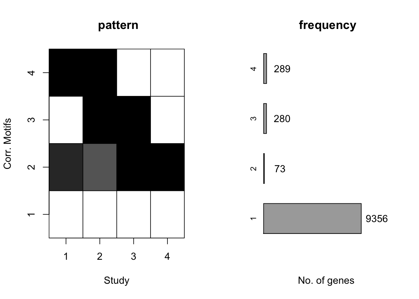
The result matches well with \(Wei\) \(and\) \(Ji\) (2015).
Simulation 2
In simulation 2, we generated 10,000 genes and four studies according to the four different patterns: 300 genes were differentially expressed in all four studies (\(Y_i = [1,1,1,1]\)); 300 genes were differential only in studies 1 and 2 (\(Y_i = [1,1,0,0]\)); 300 genes were differential only in studies 3 and 4 (\(Y_i = [0,0,1,1]\)); 9100 genes were non-differential (\(Y_i = [0,0,0,0]\)).
K = 4
D = 4
G = 10000
pi0 = c(0.03,0.03,0.03,0.91)
q0 = matrix(0,nrow=K,ncol=D)
q0[1,] = c(1,1,1,1)
q0[2,] = c(1,1,0,0)
q0[3,] = c(0,0,1,1)
q0[4,] = c(0,0,0,0)
X = matrix(0,nrow=G,ncol=6*D)
rows = rep(1:K,times=pi0*G)
A = q0[rows,]
set.seed(2)
for(g in 1:G){
  for(d in 1:D){
    sigma2 = 4*0.02/rchisq(1,4)
    x = rnorm(6,0,sqrt(sigma2))
    if(A[g,d]==1){
      dx = rnorm(1,0,4*sqrt(sigma2))
      x[1:3] = x[1:3]+dx
    }
    X[g,(6*d-5):(6*d)] = x
  }
}
groupid = rep(1:8,each=3)
compgroup = t(matrix(1:8,ncol=4))
motif.fitted<-cormotiffit(X,groupid,compgroup,K=1:5,max.iter=1000,BIC=TRUE)
[1] "We have run the first 50 iterations for K=3"
[1] "We have run the first 50 iterations for K=4"
[1] "We have run the first 100 iterations for K=4"
[1] "We have run the first 150 iterations for K=4"
[1] "We have run the first 200 iterations for K=4"
[1] "We have run the first 250 iterations for K=4"
[1] "We have run the first 300 iterations for K=4"
[1] "We have run the first 350 iterations for K=4"
[1] "We have run the first 50 iterations for K=5"
[1] "We have run the first 100 iterations for K=5"
[1] "We have run the first 150 iterations for K=5"
[1] "We have run the first 200 iterations for K=5"
[1] "We have run the first 250 iterations for K=5"
[1] "We have run the first 300 iterations for K=5"
[1] "We have run the first 350 iterations for K=5"
[1] "We have run the first 400 iterations for K=5"
[1] "We have run the first 450 iterations for K=5"
[1] "We have run the first 500 iterations for K=5"
[1] "We have run the first 550 iterations for K=5"
[1] "We have run the first 600 iterations for K=5"
[1] "We have run the first 650 iterations for K=5"
[1] "We have run the first 700 iterations for K=5"
[1] "We have run the first 750 iterations for K=5"
[1] "We have run the first 800 iterations for K=5"plotIC(motif.fitted)
plotMotif(motif.fitted)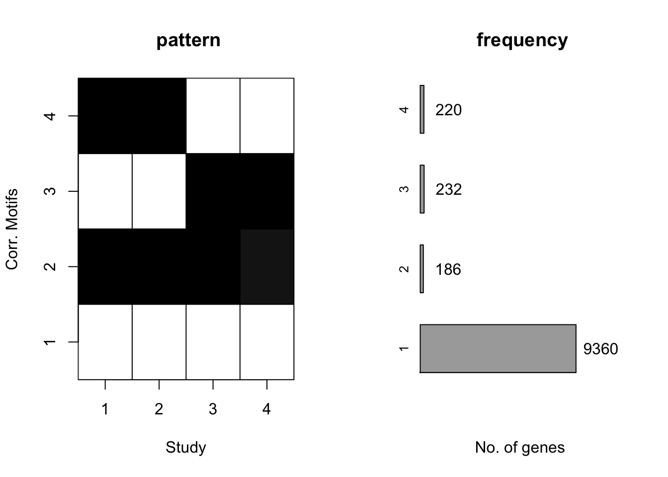
Then we could check if we change the proportion of four patterns to \(200:50:50:9700\).
K = 4
D = 4
G = 10000
pi0 = c(0.02,0.005,0.005,0.97)
q0 = matrix(0,nrow=K,ncol=D)
q0[1,] = c(1,1,1,1)
q0[2,] = c(1,1,0,0)
q0[3,] = c(0,0,1,1)
q0[4,] = c(0,0,0,0)
X = matrix(0,nrow=G,ncol=6*D)
rows = rep(1:K,times=pi0*G)
A = q0[rows,]
set.seed(1)
for(g in 1:G){
  for(d in 1:D){
    sigma2 = 4*0.02/rchisq(1,4)
    x = rnorm(6,0,sqrt(sigma2))
    if(A[g,d]==1){
      dx = rnorm(1,0,4*sqrt(sigma2))
      x[1:3] = x[1:3]+dx
    }
    X[g,(6*d-5):(6*d)] = x
  }
}
groupid = rep(1:8,each=3)
compgroup = t(matrix(1:8,ncol=4))
motif.fitted<-cormotiffit(X,groupid,compgroup,K=1:5,max.iter=1000,BIC=TRUE)
[1] "We have run the first 50 iterations for K=3"
[1] "We have run the first 100 iterations for K=3"
[1] "We have run the first 150 iterations for K=3"
[1] "We have run the first 200 iterations for K=3"
[1] "We have run the first 50 iterations for K=4"
[1] "We have run the first 100 iterations for K=4"
[1] "We have run the first 150 iterations for K=4"
[1] "We have run the first 200 iterations for K=4"
[1] "We have run the first 250 iterations for K=4"
[1] "We have run the first 300 iterations for K=4"
[1] "We have run the first 350 iterations for K=4"
[1] "We have run the first 50 iterations for K=5"
[1] "We have run the first 100 iterations for K=5"
[1] "We have run the first 150 iterations for K=5"
[1] "We have run the first 200 iterations for K=5"
[1] "We have run the first 250 iterations for K=5"
[1] "We have run the first 300 iterations for K=5"
[1] "We have run the first 350 iterations for K=5"
[1] "We have run the first 400 iterations for K=5"
[1] "We have run the first 450 iterations for K=5"
[1] "We have run the first 500 iterations for K=5"
[1] "We have run the first 550 iterations for K=5"
[1] "We have run the first 600 iterations for K=5"
[1] "We have run the first 650 iterations for K=5"
[1] "We have run the first 700 iterations for K=5"plotIC(motif.fitted)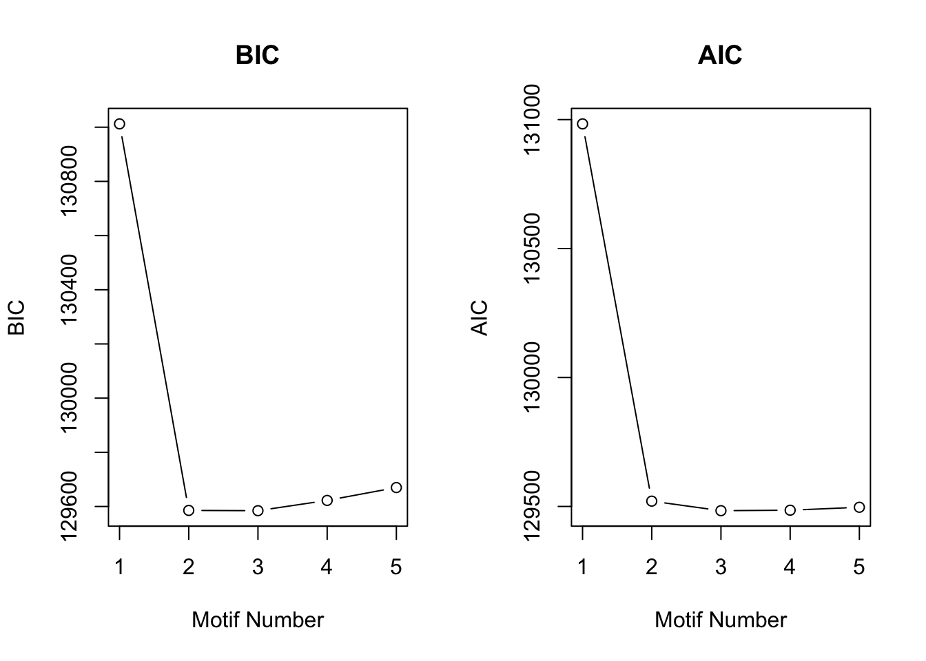
plotMotif(motif.fitted)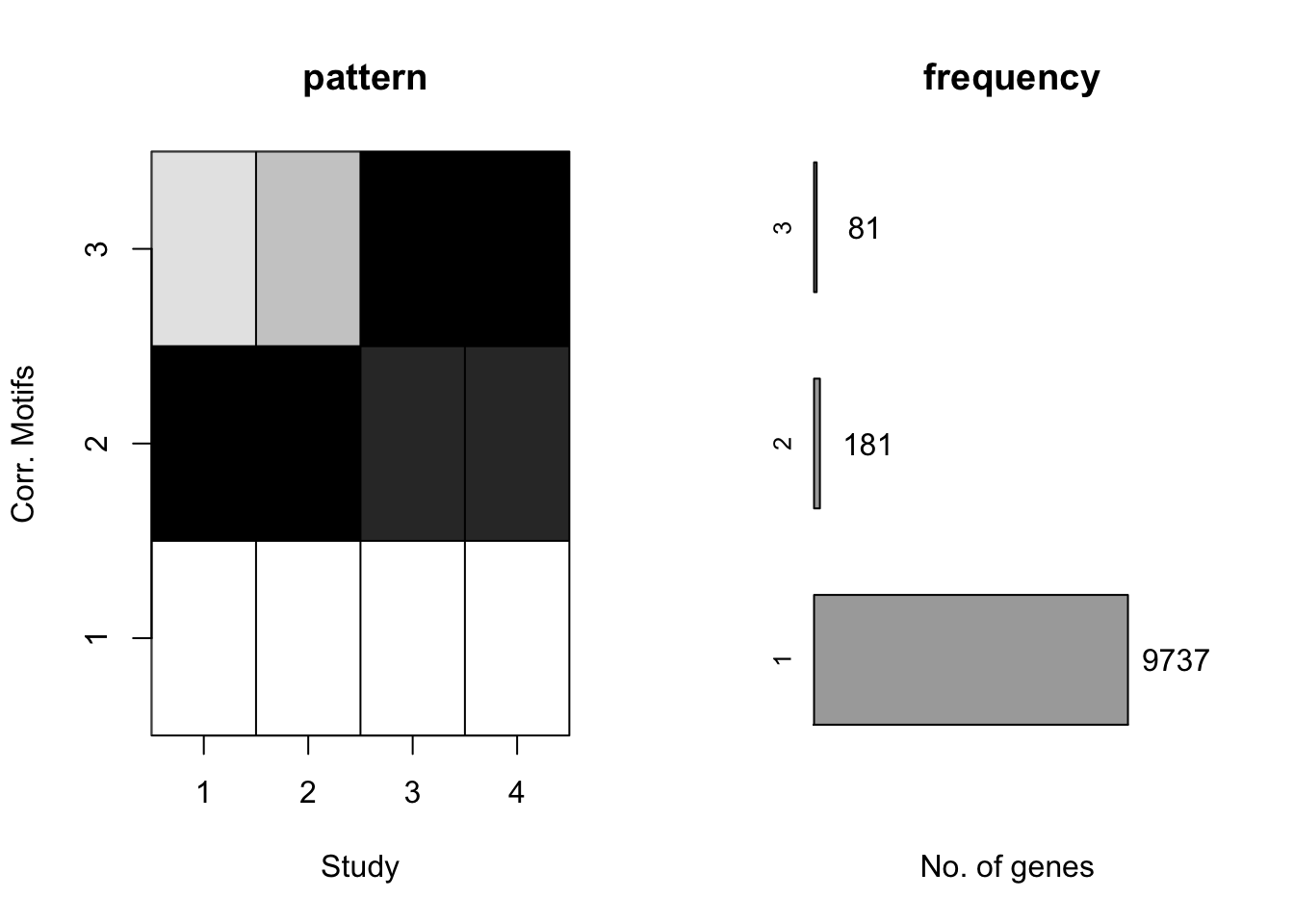
We could find that the second and third pattern merged togethor, since their proportions were relatively small compared to the first and forth pattern.
Simulation 3
In simulation 3, we generated 10,000 genes and eight studies according to the four different patterns: 200 genes were differentially expressed in all four studies (\(Y_i = [1,1,1,1,1,1,1,1]\)); 200 genes were differential only in studies 1, 2, 3, 4 (\(Y_i = [1,1,1,1,0,0,0,0]\)); 200 genes were differential only in studies 5, 6, 7, 8 (\(Y_i = [0,0,0,0,1,1,1,1]\)); 200 genes were differential only in studies 3, 4, 5, 6 (\(Y_i = [0,0,1,1,1,1,0,0]\)); 9200 genes were non-differential (\(Y_i = [0,0,0,0,0,0,0,0,0]\)).
K = 5
D = 8
G = 10000
pi0 = c(0.02,0.02,0.02,0.02,0.92)
q0 = matrix(0,nrow=K,ncol=D)
q0[1,] = c(1,1,1,1,1,1,1,1)
q0[2,] = c(1,1,1,1,0,0,0,0)
q0[3,] = c(0,0,0,0,1,1,1,1)
q0[4,] = c(0,0,1,1,1,1,0,0)
q0[5,] = c(0,0,0,0,0,0,0,0)
X = matrix(0,nrow=G,ncol=6*D)
rows = rep(1:K,times=pi0*G)
A = q0[rows,]
set.seed(3)
for(g in 1:G){
  for(d in 1:D){
    sigma2 = 4*0.02/rchisq(1,4)
    x = rnorm(6,0,sqrt(sigma2))
    if(A[g,d]==1){
      dx = rnorm(1,0,4*sqrt(sigma2))
      x[1:3] = x[1:3]+dx
    }
    X[g,(6*d-5):(6*d)] = x
  }
}
groupid = rep(1:16,each=3)
compgroup = t(matrix(1:16,nrow=2))
motif.fitted<-cormotiffit(X,groupid,compgroup,K=1:6,max.iter=1000,BIC=TRUE)
[1] "We have run the first 50 iterations for K=3"
[1] "We have run the first 50 iterations for K=4"
[1] "We have run the first 50 iterations for K=5"
[1] "We have run the first 50 iterations for K=6"
[1] "We have run the first 100 iterations for K=6"plotIC(motif.fitted)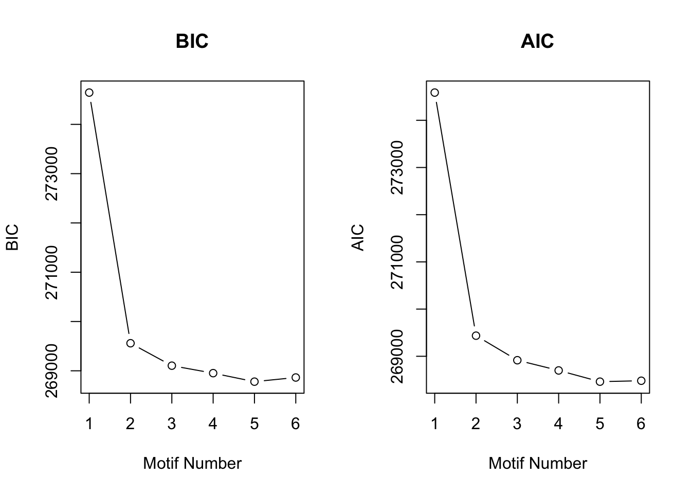
plotMotif(motif.fitted)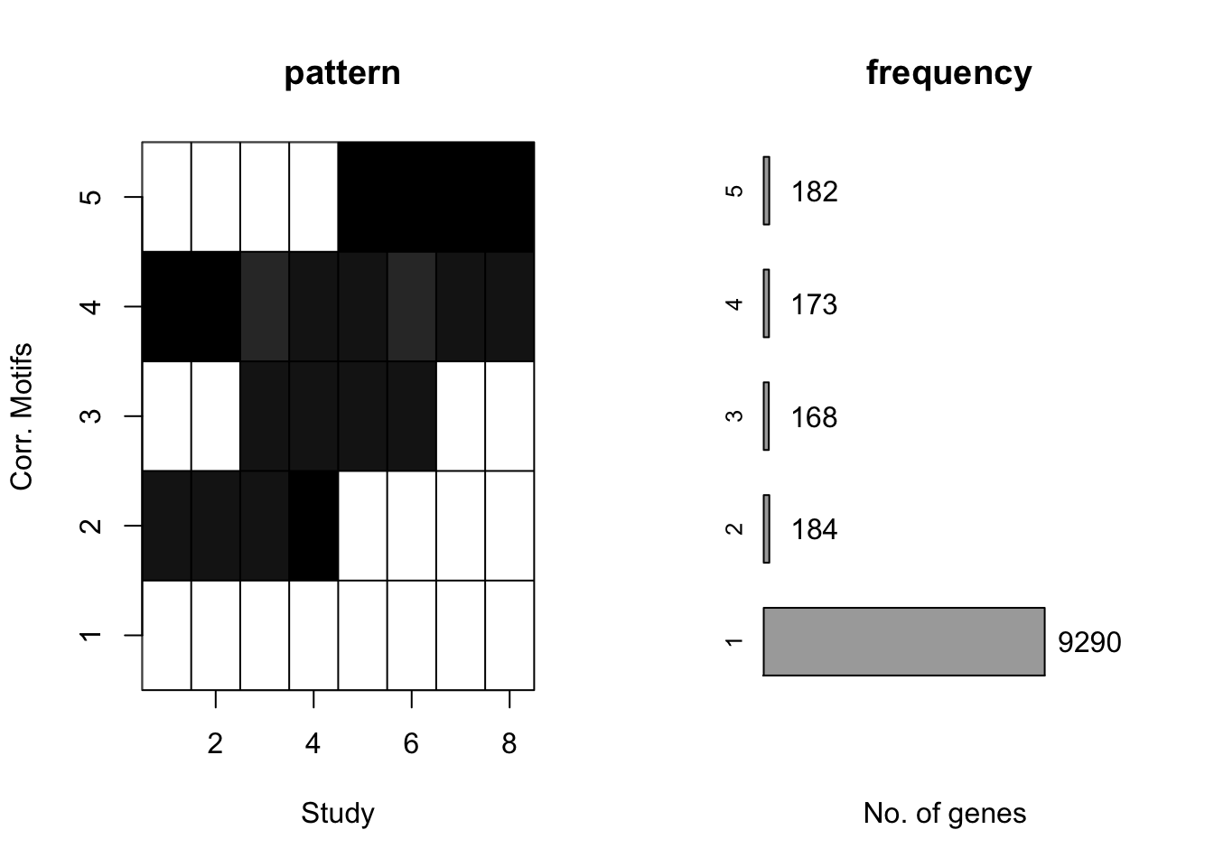
CorMotif tends to merge weaker patterns with small proportion. Just as \(Wei\) \(and\) \(Ji\) (2015) states, correlation motifs only represent a parsimonious representation of the correlation structure supported by the available data. On the other hand, the two stage method may also be blame. Adding \(limma\) structure can increase inaccuracy for estimation. In the next section, we will generate \(x_{ir}\) directly from a Gaussian distribution. In fact, any distribution can be applied under our framework. In addition, we can also estimate the parameters for Gaussian distribution.
CorMotif based on Gaussian model
Let
\[\begin{eqnarray*} f_{r0}(x_{ir}) &=& N(x_{ir};0,1), \\ f_{r1}(x_{ir}) &=& N(x_{ir};0,1+\sigma_r^2). \end{eqnarray*}\]First, we checked the performance of CorMotif by assuming we know \(\sigma^2\) exactly. Then we dealed with the situation where we were given no information about \(\sigma^2\). Apply
\[\sigma_r^{2(t+1)}= \frac{\sum_{i=1}^n \sum_{k=1}^K (x_{ir}^2-1)p_{ikr1}}{\sum_{i=1}^n \sum_{k=1}^K p_{ikr1}},\]
from my write-up document, we could iteratively update \(\sigma_r^2\).
Simulation 4
We used the same patterns and proportions as Simulation 1 in the previous section and let \(\sigma^2=(4^2,4^2,4^2,4^2)\). Assume we know \(\sigma^2\), the estimated results were:
K = 4
D = 4
G = 10000
sigma2 = c(16,16,16,16)
pi0 = c(0.01,0.04,0.04,0.91)
q0 = matrix(0,nrow=K,ncol=D)
q0[1,] = c(1,1,1,1)
q0[2,] = c(1,1,0,0)
q0[3,] = c(0,1,1,0)
q0[4,] = c(0,0,0,0)
X = matrix(0,nrow=G,ncol=D)
rows = rep(1:K,times=pi0*G)
A = q0[rows,]
set.seed(4)
for(g in 1:G){
  for(d in 1:D){
    if(A[g,d]==1){
      X[g,d] = rnorm(1,0,sqrt(1+sigma2[d]))
    } else{
      X[g,d] = rnorm(1,0,1)
    }
  }
}
motif.fitted<-cormotiffit.norm.known(X,sigma2,K=1:5,max.iter=1000,BIC=TRUE)
plotIC(motif.fitted)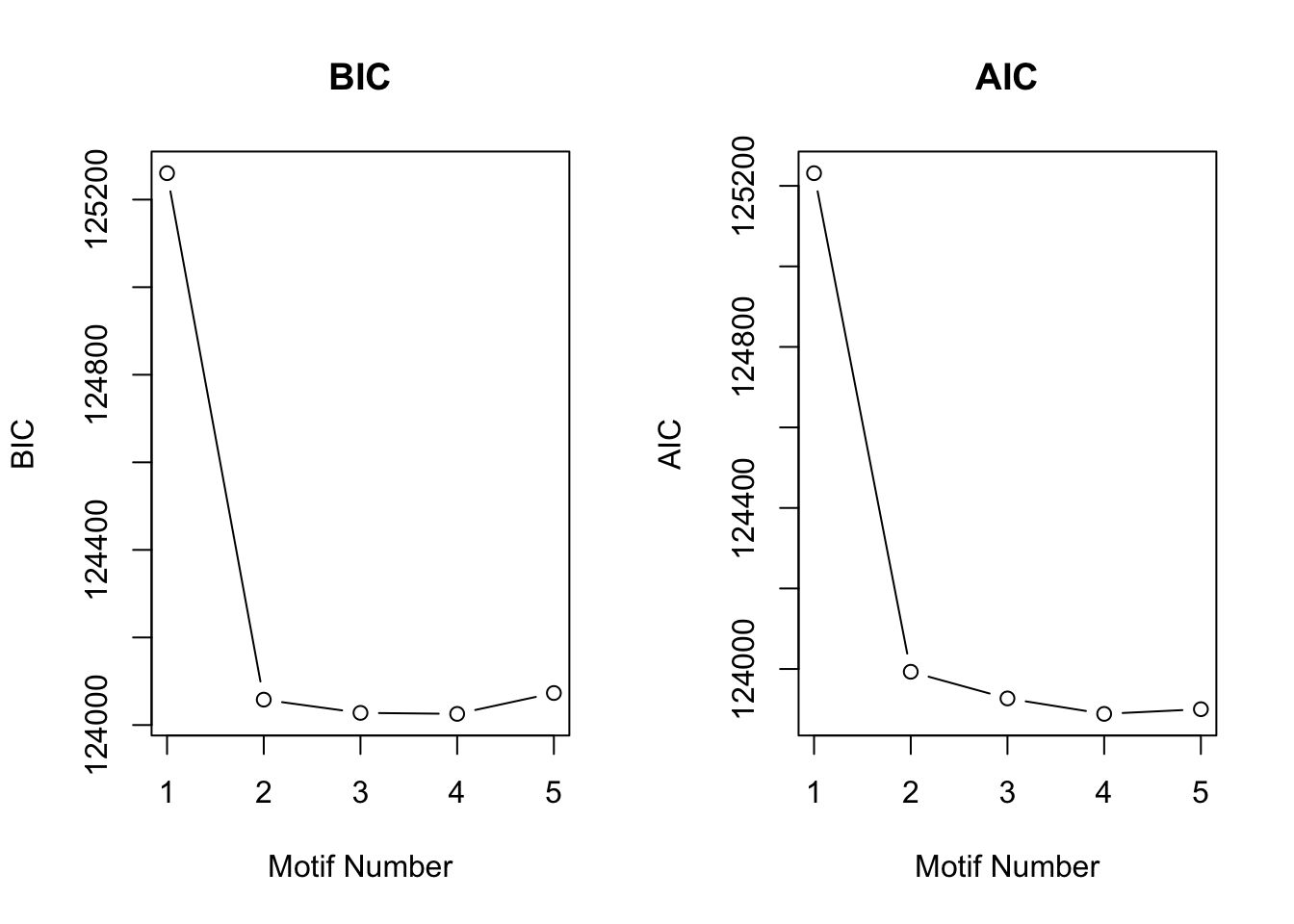
plotMotif(motif.fitted)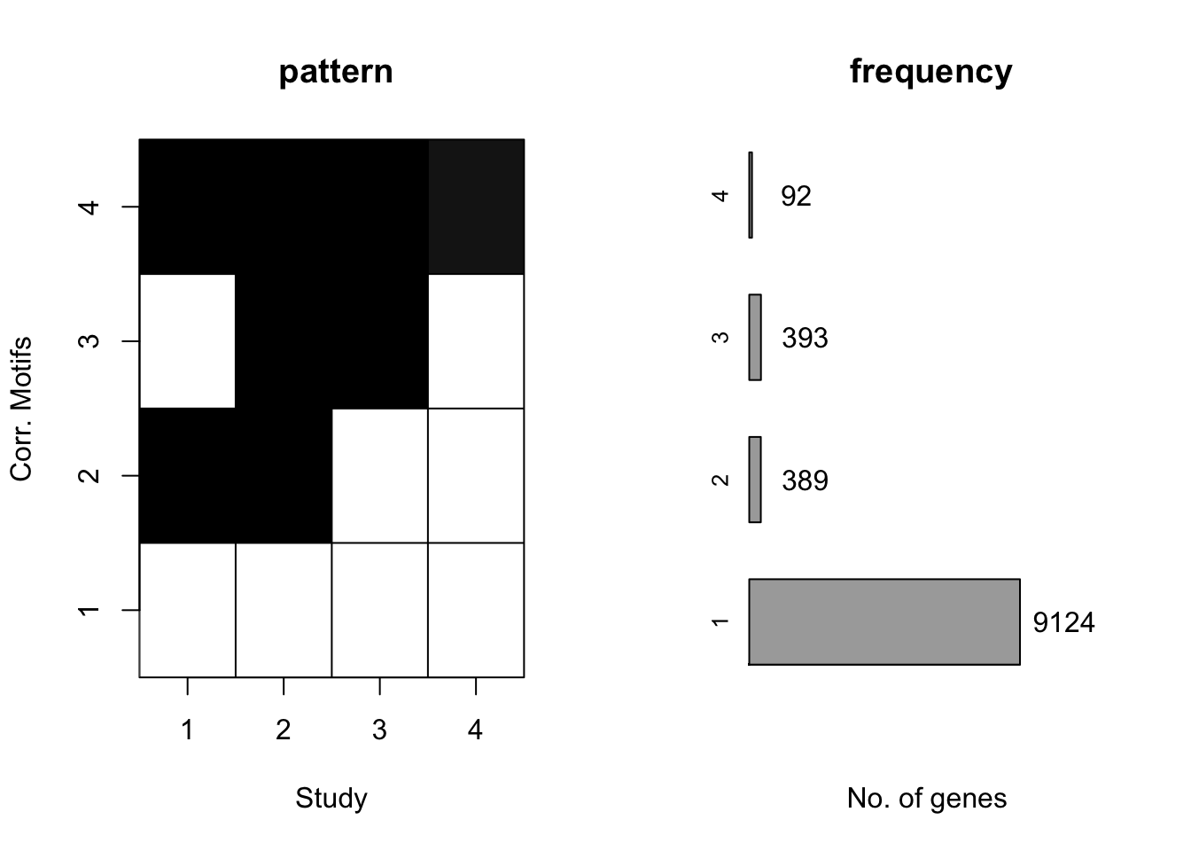
CorMotif could correctly recognize four patterns and the proportion is also reasonable. Then we checked the performace without any prior information about \(\sigma^2\) with the same simulated data.
motif.fitted<-cormotiffit.norm(X,K=1:5,max.iter=1000,BIC=TRUE)
plotIC(motif.fitted)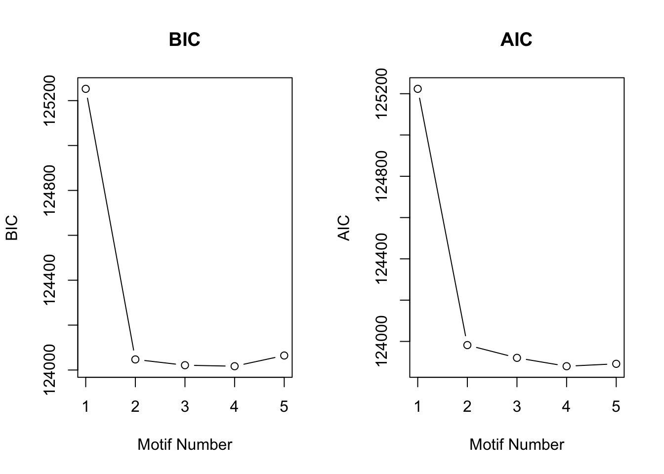
plotMotif(motif.fitted)
And the estimated \(\sigma^2\) is
motif.fitted$bestmotif$motif.s[1] 15.57719 17.97454 14.37695 10.53775Simulation 5
We used the same patterns and proportions as Simulation 2 in the previous section and let \(\sigma^2=(4^2,4^2,4^2,4^2)\). Assume we know \(\sigma^2\), the estimated results were:
K = 4
D = 4
G = 10000
sigma2 = c(16,16,16,16)
pi0 = c(0.03,0.03,0.03,0.91)
q0 = matrix(0,nrow=K,ncol=D)
q0[1,] = c(1,1,1,1)
q0[2,] = c(1,1,0,0)
q0[3,] = c(0,0,1,1)
q0[4,] = c(0,0,0,0)
X = matrix(0,nrow=G,ncol=D)
rows = rep(1:K,times=pi0*G)
A = q0[rows,]
set.seed(4)
for(g in 1:G){
  for(d in 1:D){
    if(A[g,d]==1){
      X[g,d] = rnorm(1,0,sqrt(1+sigma2[d]))
    } else{
      X[g,d] = rnorm(1,0,1)
    }
  }
}
motif.fitted<-cormotiffit.norm.known(X,sigma2,K=1:5,max.iter=1000,BIC=TRUE)
plotIC(motif.fitted)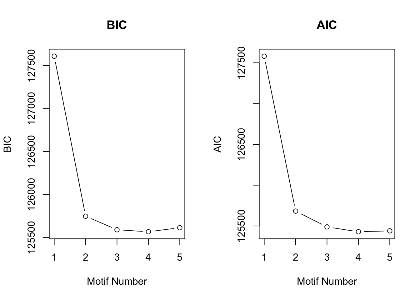
plotMotif(motif.fitted)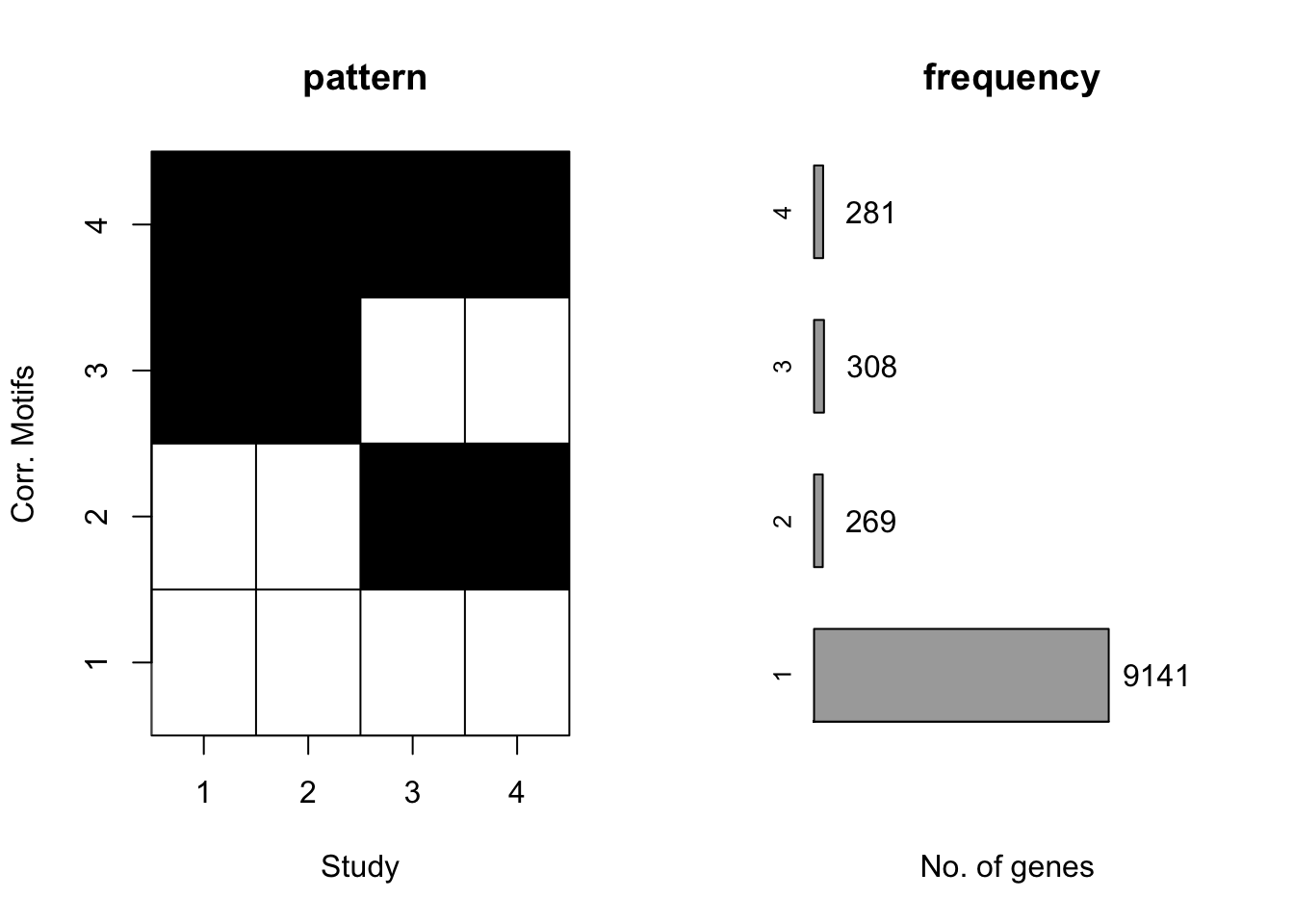
Again, CorMotif could correctly recognize four patterns and the proportion is also accurate. Then we checked the performace without any prior information about \(\sigma^2\) with the same simulated data.
motif.fitted<-cormotiffit.norm(X,K=1:5,max.iter=1000,BIC=TRUE)
plotIC(motif.fitted)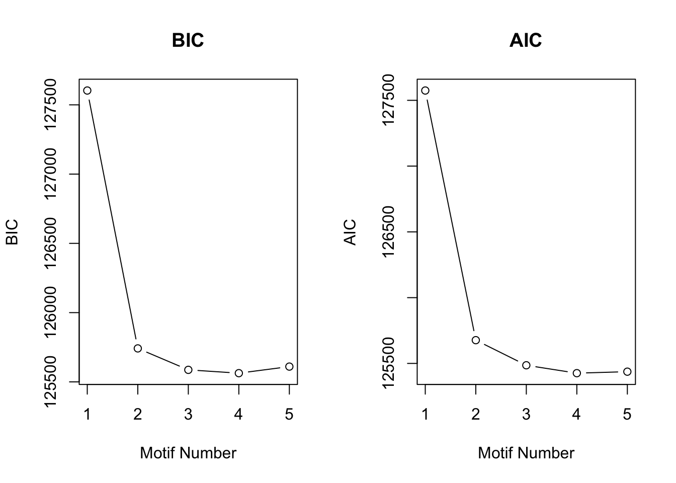
plotMotif(motif.fitted)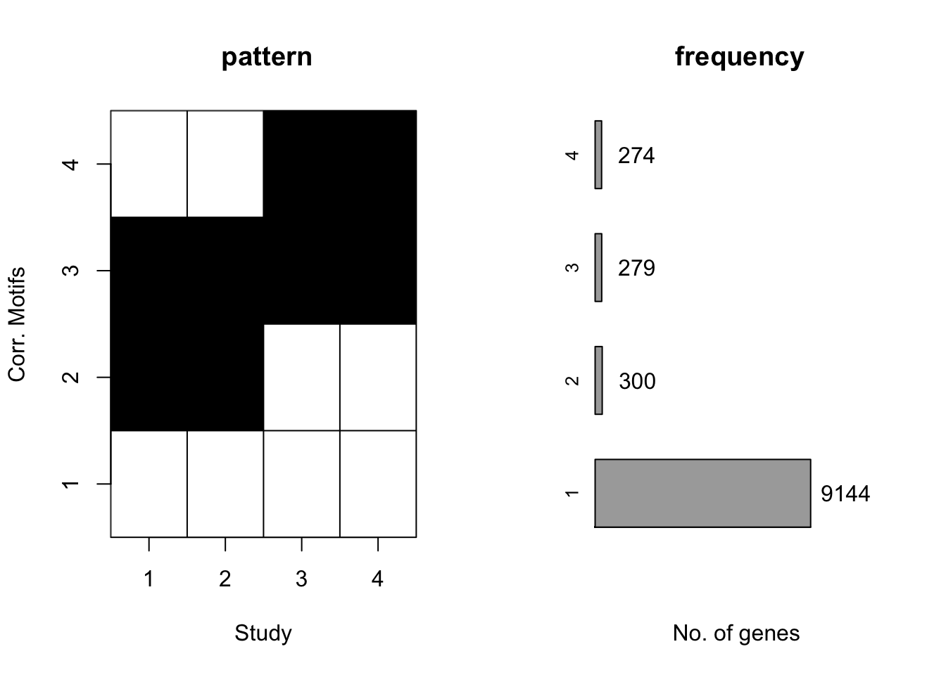
And the estimated \(\sigma^2\) is
motif.fitted$bestmotif$motif.s[1] 15.44301 17.94769 15.85088 15.46378Simulation 6
We used the same patterns and proportions as Simulation 3 in the previous section and let \(\sigma^2=(4^2,4^2,4^2,4^2,4^2,4^2,4^2,4^2)\). Assume we know \(\sigma^2\), the estimated results were:
K = 5
D = 8
G = 10000
sigma2 = rep(16,D)
pi0 = c(0.02,0.02,0.02,0.02,0.92)
q0 = matrix(0,nrow=K,ncol=D)
q0[1,] = c(1,1,1,1,1,1,1,1)
q0[2,] = c(1,1,1,1,0,0,0,0)
q0[3,] = c(0,0,0,0,1,1,1,1)
q0[4,] = c(0,0,1,1,1,1,0,0)
q0[5,] = c(0,0,0,0,0,0,0,0)
X = matrix(0,nrow=G,ncol=D)
rows = rep(1:K,times=pi0*G)
A = q0[rows,]
for(g in 1:G){
  for(d in 1:D){
    if(A[g,d]==1){
      X[g,d] = rnorm(1,0,sqrt(1+sigma2[d]))
    } else{
      X[g,d] = rnorm(1,0,1)
    }
  }
}
motif.fitted<-cormotiffit.norm.known(X,sigma2,K=1:6,max.iter=1000,BIC=TRUE)
plotIC(motif.fitted)
plotMotif(motif.fitted)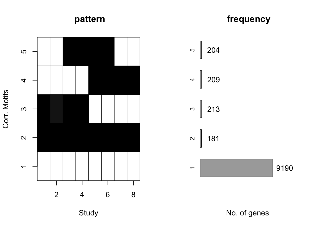
Then we checked the performace without any prior information about \(\sigma^2\) with the same simulated data.
motif.fitted<-cormotiffit.norm(X,K=1:6,max.iter=1000,BIC=TRUE)
plotIC(motif.fitted)
plotMotif(motif.fitted)
And the estimated \(\sigma^2\) is
motif.fitted$bestmotif$motif.s[1] 17.52847 16.99682 16.54558 16.10108 16.85498 16.83212 17.13306 13.94331Under all situation, CorMotif without knowing \(\sigma^2\) performed equally well with knowing \(\sigma^2\).
Discussion
We tested CorMotif for both \(limma\) and Guassion model. Through our simulation, we find that correlation motifs only represent a parsimonious representation of the correlation structure. The reason is twofold. On the one hand, CorMotif tends to merge patterns with small proportion. On the other hand, if the differences between cases and controls (for Gaussian model, the variance \(\sigma^2\)) are not significant, CorMotif cannot detect the pattern either.
Session information
print(sessionInfo())R version 3.4.1 (2017-06-30)
Platform: x86_64-apple-darwin15.6.0 (64-bit)
Running under: macOS Sierra 10.12.5
Matrix products: default
BLAS: /Library/Frameworks/R.framework/Versions/3.4/Resources/lib/libRblas.0.dylib
LAPACK: /Library/Frameworks/R.framework/Versions/3.4/Resources/lib/libRlapack.dylib
locale:
[1] en_US.UTF-8/en_US.UTF-8/en_US.UTF-8/C/en_US.UTF-8/en_US.UTF-8
attached base packages:
[1] stats graphics grDevices utils datasets methods base
loaded via a namespace (and not attached):
[1] compiler_3.4.1 backports_1.1.0 magrittr_1.5 rprojroot_1.2
[5] tools_3.4.1 htmltools_0.3.6 yaml_2.1.14 Rcpp_0.12.12
[9] stringi_1.1.5 rmarkdown_1.6 knitr_1.17 git2r_0.19.0
[13] stringr_1.2.0 digest_0.6.12 evaluate_0.10.1This R Markdown site was created with workflowr