Last updated: 2020-09-30

Checks: 6 1

Knit directory: causal-TWAS/

This reproducible R Markdown analysis was created with workflowr (version 1.6.2). The Checks tab describes the reproducibility checks that were applied when the results were created. The Past versions tab lists the development history.

R Markdown file: uncommitted changes

The R Markdown file has unstaged changes. To know which version of the R Markdown file created these results, you’ll want to first commit it to the Git repo. If you’re still working on the analysis, you can ignore this warning. When you’re finished, you can run wflow_publish to commit the R Markdown file and build the HTML.

Environment: empty

Great job! The global environment was empty. Objects defined in the global environment can affect the analysis in your R Markdown file in unknown ways. For reproduciblity it’s best to always run the code in an empty environment.

Seed: set.seed(20191103)

The command set.seed(20191103) was run prior to running the code in the R Markdown file. Setting a seed ensures that any results that rely on randomness, e.g. subsampling or permutations, are reproducible.

Session information: recorded

Great job! Recording the operating system, R version, and package versions is critical for reproducibility.

Cache: none

Nice! There were no cached chunks for this analysis, so you can be confident that you successfully produced the results during this run.

File paths: relative

Great job! Using relative paths to the files within your workflowr project makes it easier to run your code on other machines.

Repository version: 69a2458

Great! You are using Git for version control. Tracking code development and connecting the code version to the results is critical for reproducibility.

The results in this page were generated with repository version 69a2458. See the Past versions tab to see a history of the changes made to the R Markdown and HTML files.

Note that you need to be careful to ensure that all relevant files for the analysis have been committed to Git prior to generating the results (you can use wflow_publish or wflow_git_commit). workflowr only checks the R Markdown file, but you know if there are other scripts or data files that it depends on. Below is the status of the Git repository when the results were generated:


Ignored files:
    Ignored:    .Rhistory
    Ignored:    .Rproj.user/
    Ignored:    code/workflow/.ipynb_checkpoints/
    Ignored:    data/

Untracked files:
    Untracked:  code/workflow/master_run.sh
    Untracked:  code/workflow/submit_parallel_master_run.sh.sh

Unstaged changes:
    Modified:   analysis/simulation-susieI-ukbchr17to22-gtex.adipose.Rmd
    Modified:   code/run_UKB_process.R
    Modified:   code/run_simulate_data.R
    Modified:   code/run_test_susieI.R
    Deleted:    code/run_test_susieI_m.R
    Modified:   code/susie_filter.R
    Modified:   code/workflow/workflow-susieI-20200813.ipynb
    Modified:   code/workflow/workflow-susieI-20200915.ipynb

Note that any generated files, e.g. HTML, png, CSS, etc., are not included in this status report because it is ok for generated content to have uncommitted changes.

These are the previous versions of the repository in which changes were made to the R Markdown (analysis/simulation-susieI-ukbchr17to22-gtex.adipose.Rmd) and HTML (docs/simulation-susieI-ukbchr17to22-gtex.adipose.html) files. If you’ve configured a remote Git repository (see ?wflow_git_remote), click on the hyperlinks in the table below to view the files as they were in that past version.

File	Version	Author	Date	Message
Rmd	34b9ed3	simingz	2020-09-18	BF
html	34b9ed3	simingz	2020-09-18	BF
Rmd	c1c6bcc	simingz	2020-09-14	susieI plots
html	c1c6bcc	simingz	2020-09-14	susieI plots
Rmd	4d39fd6	simingz	2020-09-14	susieI plots
html	4d39fd6	simingz	2020-09-14	susieI plots
Rmd	79b77d5	simingz	2020-09-04	susieI more runs
html	79b77d5	simingz	2020-09-04	susieI more runs
Rmd	bb0bce0	simingz	2020-09-03	susie prior
html	bb0bce0	simingz	2020-09-03	susie prior
Rmd	193a8df	simingz	2020-09-01	increase gene pve
html	193a8df	simingz	2020-09-01	increase gene pve
Rmd	86681eb	simingz	2020-08-28	susieI all regions
html	86681eb	simingz	2020-08-28	susieI all regions
Rmd	41c8849	simingz	2020-08-20	more parameter examples for susieI
html	41c8849	simingz	2020-08-20	more parameter examples for susieI
Rmd	86ac96e	simingz	2020-08-19	more iterations
html	86ac96e	simingz	2020-08-19	more iterations
Rmd	bd402eb	simingz	2020-08-19	susieI bug fix
html	bd402eb	simingz	2020-08-19	susieI bug fix
Rmd	f125882	simingz	2020-08-19	susieI
html	f125882	simingz	2020-08-19	susieI
Rmd	d299f60	simingz	2020-08-19	susieI
html	d299f60	simingz	2020-08-19	susieI
Rmd	846fb96	simingz	2020-08-14	susieI
html	846fb96	simingz	2020-08-14	susieI
Rmd	fd909a1	simingz	2020-08-14	susieI

library(mr.ash.alpha)
library(data.table)
suppressMessages({library(plotly)})
library(tidyr)
library(plyr)
library(stringr)
library(kableExtra)
source("analysis/summarize_twas_plots.R")

Analysis description

n <- 20000 # number of samples
p <- 86000 # number of SNPs
J <- 1653 # number of genes

The genotype data we used is from UKB biobank, randomly selecting n = 20000 samples. We use SNP genotype data from chr 17 to chr 22 combined. These genomic regions represents 12.5% of the genome. SNPs are downsampled to 1/10 (randomly), eQTLs (see below for definition of eQTL) were added back. This ends up with p = p as.charater(p) SNPs.

Our analysis consists of the following steps:

Build expression predictors using another expression-genotype dataset.

The one we used in this analysis is GTEx Adipose tissue v7 dataset. This dataset contains ~ 380 samples. FUSION/TWAS were used to train expression model and we used their lasso results. SNPs included in eQTL anlaysis are restricted to cis-locus 500kb on either side of the gene boundary. eQTLs are defined as SNPs with abs(effectize) > 1e-8 in lasso results.

Impute expression.

We impute gene expression for our genotype data using expression models obtained from step 1. There are 1653 genes with expression model from chr17 to chr22. We imputed expression from genotypes using the expression predictors.

Define and select regions

Next, the analysis is done at the “region” level, which is 500kb bins along the genome. Each bin would contain all the SNPs, as well as all the genes in that bin. We are exploring several ways to select regions that contain true signals, e.g. based on regional sum of mr.ash PIP for genes/SNPs, region smallest TWAS p value for gene/SNPs, or regional bayes factors, etc.

Run susie iteratively We then run susie for each of these regions. So the features of SuSiE are: SNPs and “genes” (not cis-eQTLs of that gene). We use the same prior for all SNPs and another prior for all “genes” when running SUSIE. In some settings, we also run SUSIE with null weight, which is calculated as 1- prior.SNP * n.SNP - prior.gene * n.gene. We obtain the PIP for SNPs and gene in the region. After we run susie for all regions (one iteration), we take the average of all SNP PIPs as the prior of SNPs for the next iteration and similarly for the prior for genes.
We obtain PIP for genes from the last iteration as results.

simdatadir <- "~/causalTWAS/simulations/simulation_ashtest_20200721/"
outputdir <- "~/causalTWAS/simulations/simulation_susieI_20200813/"
susiedir <- "~/causalTWAS/simulations/simulation_susieI_20200813/"
mrashdir <- "~/causalTWAS/simulations/simulation_ashtest_20200721/"
tag <- '20200813-1-1'
Niter <- 30

Regional minimum p value distribution

minimum TWAS p value of genes for each region:

simtag <- "20200721-1-1"
rpipf <- paste0(simdatadir, simtag, ".pgenerprank.txt")

a <- read.table(rpipf, header = T)
a.c <- a[a$nCausal > 0, ]
ax <- pretty(0:max(-log10(a$rpmin)), n = 30)

par(mfrow=c(2,1))
h1 <- hist(-log10(a$rpmin), breaks = 100, xlab = "PIP", main = "min P value distribution-all", col = "grey"); grid()
h2 <- hist(-log10(a.c$rpmin), breaks = h1$breaks, xlab = "PIP", main = "min p distribution-causal", col = "salmon");grid()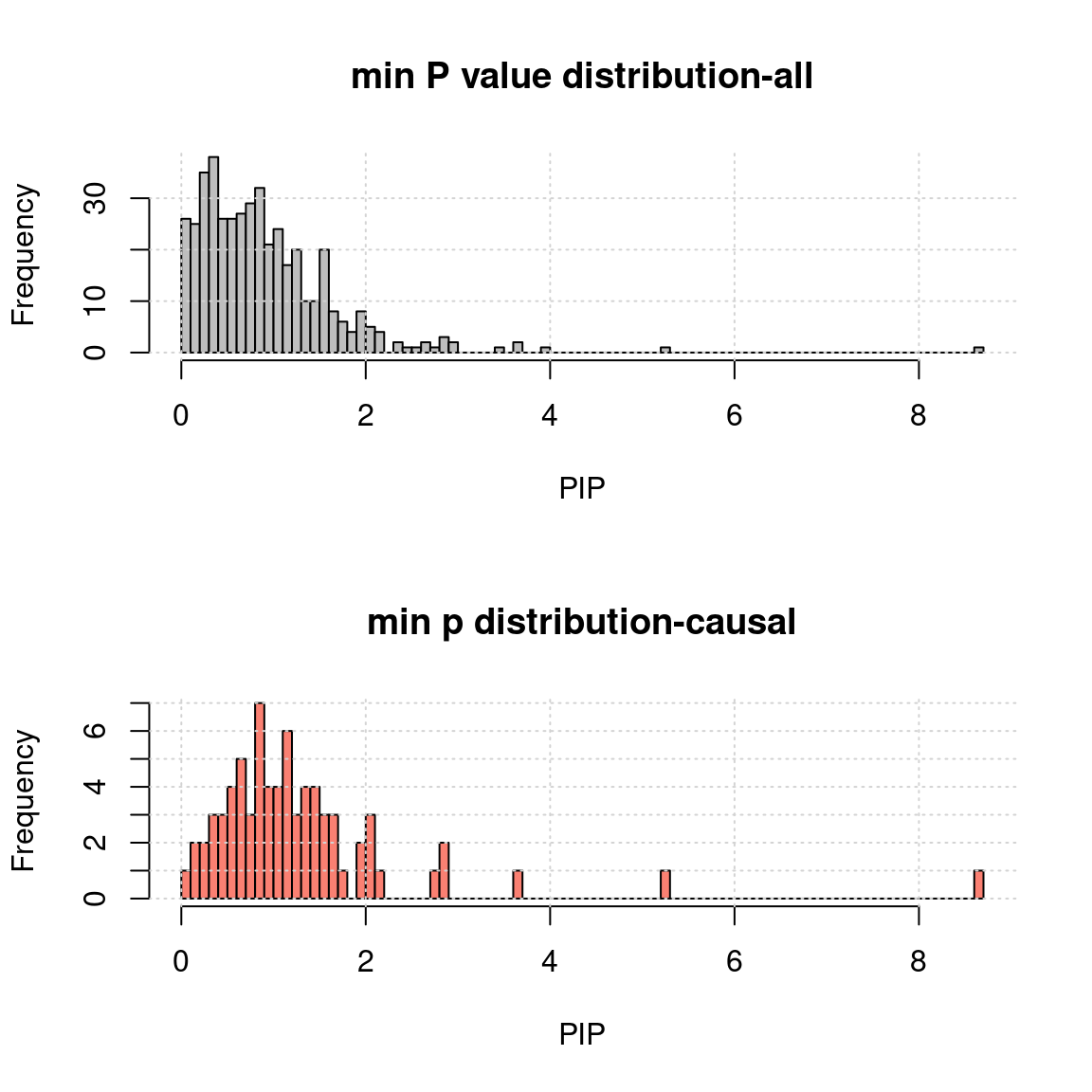

Version	Author	Date
4d39fd6	simingz	2020-09-14

minimum TWAS p value of genes and SNPs for each region:

rpipf <- paste0(simdatadir, simtag, ".p2rprank.txt")

a <- read.table(rpipf, header = T)
a.c <- a[a$nCausal > 0, ]
ax <- pretty(0:max(-log10(a$rpmin)), n = 30)

par(mfrow=c(2,1))
h1 <- hist(-log10(a$rpmin), breaks = 100, xlab = "PIP", main = "min P value distribution-all", col = "grey"); grid()
h2 <- hist(-log10(a.c$rpmin), breaks = h1$breaks, xlab = "PIP", main = "min p distribution-causal", col = "salmon");grid()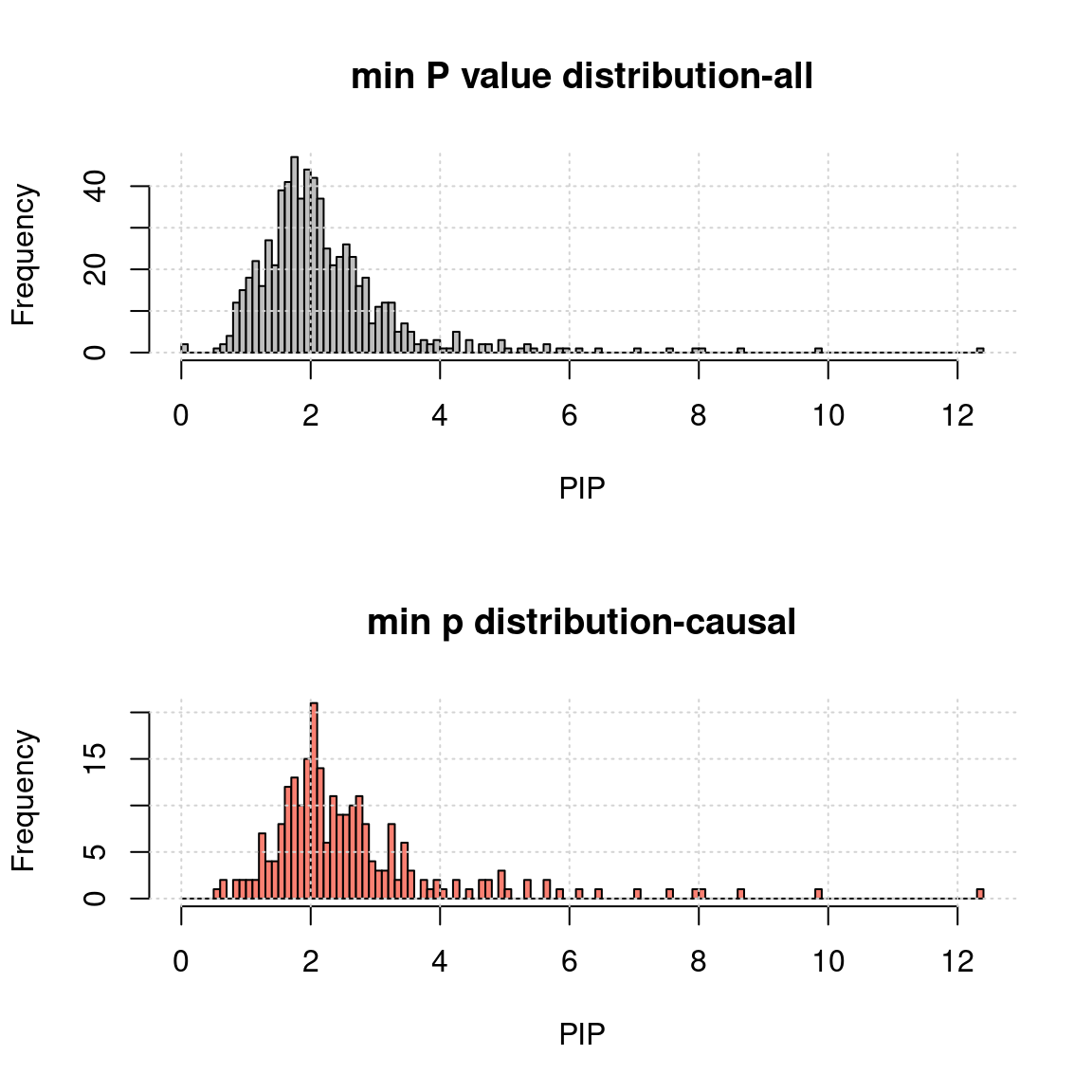

Version	Author	Date
4d39fd6	simingz	2020-09-14

Regional BF distribution

mean BF of both SNPs and genes in region as the regional BF.

rpipf <- paste0(simdatadir, simtag, ".rBF.txt")

a <- read.table(rpipf, header = T)
a.c <- a[a$nCausal > 0, ]

par(mfrow=c(2,1))
h1 <- hist(a$rBF, breaks = 5000, xlab = "PIP", main = "regional BF distribution-all", col = "grey", xlim = c(0,10)); grid()
h2 <- hist(a.c$rBF, breaks = h1$breaks, xlab = "PIP", main = "regional BF distribution-causal", col = "salmon",xlim = c(0,10));grid()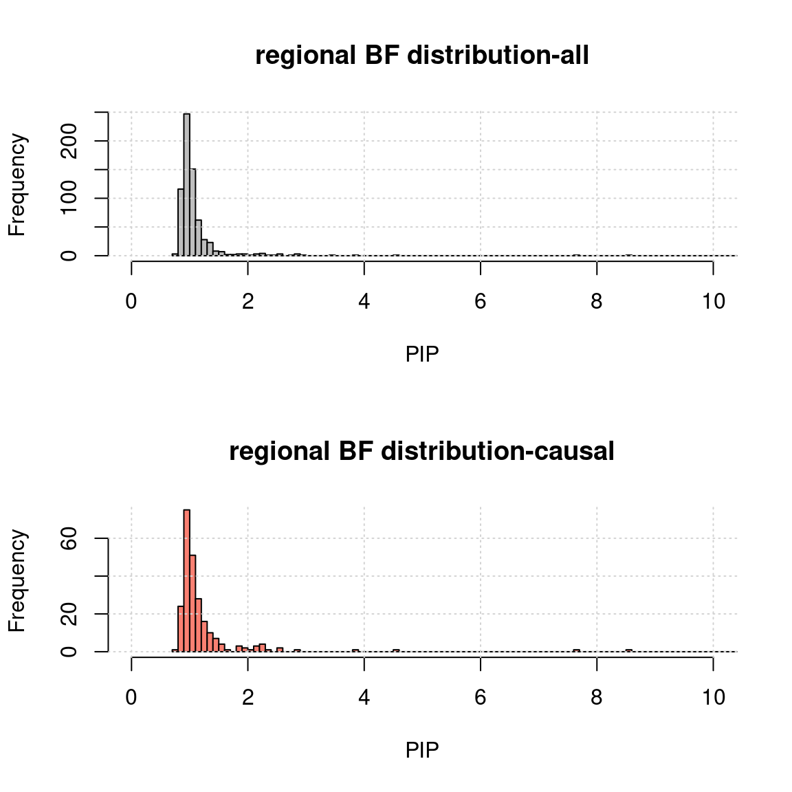

Version	Author	Date
34b9ed3	simingz	2020-09-18

MR.ASH regional pip sum distribution

Use mr.ash for gene only:

rpipf <- paste0(simdatadir, simtag, "-mr.ash.mrashrPIP.txt")

a <- read.table(rpipf, header = T)
a.c <- a[a$nCausal > 0, ]
ax <- pretty(0:max(a$rPIP), n = 30)

par(mfrow=c(2,1))
h1 <- hist(a$rPIP, breaks = 100, xlab = "PIP", main = "PIP distribution-all", col = "grey"); grid()
h2 <- hist(a.c$rPIP, breaks = h1$breaks, xlab = "PIP", main = "PIP distribution-causal", col = "salmon");grid()

MR.ash2s for both genes and SNPs using the same data

rpipf <- paste0(simdatadir, simtag, "-mr.ash2s.lassoes-es.mrash2srPIP.txt")

a <- read.table(rpipf, header = T)
a.c <- a[a$nCausal > 0 ,]
ax <- pretty(0:max(a$rPIP), n = 30) # Make a neat vector for the breakpoints

par(mfrow=c(2,1))
h1 <- hist(a$rPIP, breaks = 100, xlab = "PIP", main = "PIP distribution-all", col = "grey"); grid()
h2 <- hist(a.c$rPIP, breaks = h1$breaks, xlab = "PIP", main = "PIP distribution-causal", col = "salmon");grid()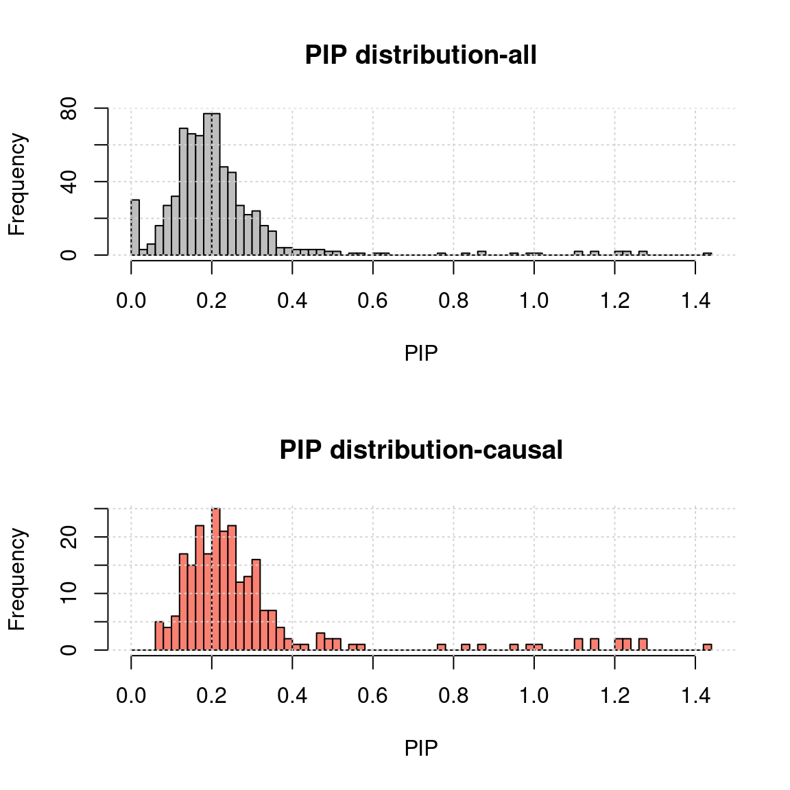

Version	Author	Date
d299f60	simingz	2020-08-19
846fb96	simingz	2020-08-14

Parameter estimation results

Results: Each row shows parameter estimation results from 5 simulation runs with similar settings (i.e. pi1 and PVE for genes and SNPs). each row has two plots, one for gene pi1 estimation, one for enrichment (gene pi1/snp pi1). Results from each run were represented by one dot, dots with the same color come from the same run. horizontal dash lines: simulation truth, mr.ash2, mr.ash for gene and SNPs; susietruth, the truth in selected regions that were used to run susie iteractively (susieI).

Regions: causal

Regions: We use regional PIP of both SNP and gene from mr.ash2s > 0.3, and also require at least one causal gene or SNP is present, also, at least one gene.
Susie run parameters: L=1, null_weight = 0, didn’t update null_weight in iterations. We initialize with prior for genes and SNPs as uniform.

show_param <- function(mrashfs, susieIfs, susieIfs2){
  param <- do.call(rbind, lapply(mr.ashfs, function(x) t(read.table(x))[2:1,]))
 
  pars <- cbind(param[seq(1,nrow(param), 2), 2], param[seq(1,nrow(param), 2), 4], param[seq(1,nrow(param), 2), 1], param[seq(2,nrow(param), 2), 1], param[seq(1,nrow(param), 2), 3], param[seq(2,nrow(param), 2), 3])
  colnames(pars) <- c("PVE.gene_truth", "PVE.SNP_truth", paste(rep(c("pi1.gene_", "pi1.SNP_"), each = 2), c("truth", "mr.ash2"), sep = ""))
    
  param.s <- do.call(rbind, lapply(susieIfs, function(x) {load(x); c(tail(prior.gene_rec, 1), tail(prior.SNP_rec,1))}))
  
  param.s.truth <- do.call(rbind, lapply(susieIfs2, function(x) {
    a <- read.table(x, header = T);
    c(nrow(a[a$ifcausal == 1 & a$type == "gene", , drop = F])/ nrow(a[a$type == "gene", , drop = F]),
      nrow(a[a$ifcausal == 1 & a$type == "SNP", , drop = F])/ nrow(a[a$type == "SNP", , drop = F]))
    }))
  
  pars.s <- cbind(param.s.truth, param.s)[, c(1,3,2,4)]
  colnames(pars.s) <-  paste(rep(c("pi1.gene_", "pi1.SNP_"), each = 2), c("susietruth", "susieI"), sep = "")
  
  df <- cbind(tags, format(pars, digits = 4), format(pars.s, digits =4))
  rownames(df) <- NULL
  return(df)
  
  # df %>% 
  # kable("html", escape = F) %>%
  # kable_styling("striped", full_width = F) %>%
  #  row_spec(c(1:5, 11:15), background = "#FEF3B9") %>%
  # scroll_box(width = "100%", height = "600px", fixed_thead = T)
}

plot_param <- function(df, ...){
  df <- apply(df[ , 2:ncol(df)], 2, function(x) as.numeric(x))
  m <- cbind(df[,"pi1.gene_mr.ash2"], 1:nrow(df), 1 + 1:nrow(df)/nrow(df)/3)
  st <-  cbind(df[,"pi1.gene_susietruth"], 1:nrow(df), 2 + 1:nrow(df)/nrow(df)/3)
  s <- cbind(df[,"pi1.gene_susieI"], 1:nrow(df), 3 + 1:nrow(df)/nrow(df)/3)
  t <- df[1,"pi1.gene_truth"]
  dfp <- rbind(m,st,s)
  plot(dfp[,3], dfp[,1], col = dfp[,2], pch = 19, ylab = "gene pi1", xaxt = "n", xlab="", xlim = c(0.8, 3.5), frame.plot=FALSE, ylim = c(0, max(dfp[,1],t) *1.05), ...)
  axis(side=1, at=1:3, labels = FALSE, tick = F)
  text(x=1:3, 0, labels = c("mr.ash2", "susieI_truth", "susieI"), xpd = T, pos =1)
  abline(h=t, lty = 2, col= "salmon", lwd=1.5)
  grid()
  
  m <- cbind(df[,"pi1.gene_mr.ash2"]/df[,"pi1.SNP_mr.ash2"], 1:nrow(df), 1 + 1:nrow(df)/nrow(df)/3)
  st <-  cbind(df[,"pi1.gene_susietruth"]/df[,"pi1.SNP_susietruth"], 1:nrow(df), 2 + 1:nrow(df)/nrow(df)/3)
  s <- cbind(df[,"pi1.gene_susieI"]/df[,"pi1.SNP_susieI"], 1:nrow(df), 3 + 1:nrow(df)/nrow(df)/3)
  t <- df[1,"pi1.gene_truth"]/df[1,"pi1.SNP_truth"]
  dfp <- rbind(m,st,s)
  plot(dfp[,3], dfp[,1], col = dfp[,2], pch = 19, ylab = "Enrichment (gene/snp)", xaxt = "n", xlab="", xlim = c(0.8, 3.5),frame.plot=FALSE, ylim = c(0, min(max(dfp[,1],t) *1.05, 150)))
  axis(side=1, at=1:3, labels = FALSE, tick = F)
  text(x=1:3, 0, labels = c("mr.ash2", "susieI_truth", "susieI"), xpd = T, pos =1)
  abline(h= t, lty = 2, col= "darkgreen", lwd=1.5)
  grid()
}

gpip_dist <- function(susiefs, ...){
  dflist <- list()
  for (f in susiefs){
    dflist[[f]] <- read.table(f, header =T , stringsAsFactors = F)
  }
  df <- do.call(rbind, dflist)
  hist(df[df$type == "gene", "susie_pip"], xlab = "gene susie PIP", 
       breaks = 50, ylim = c(0,20), xlim=c(0,1), col = "salmon", ...)
}

tags <- paste(rep(1:3, each = 5), 1:5, sep = "-")
mr.ashfs <- paste0(mrashdir, "20200721-", tags, "-mr.ash2s.lassoes-es.param.txt")
susieIfs <- paste0(outputdir, "20200813-", tags, ".susieIres.Rd")
susieIfs2 <- paste0(outputdir, "20200813-", tags, ".1.txt")

df <- show_param(mrashfs, susieIfs, susieIfs2)
par(mfrow = c(3,2))
plot_param(df[1:5,], main = "1-x: gene.pve ~ 0.01, snp.pve ~ 0.05") 
plot_param(df[6:10,], main = "2-x: gene.pve ~ 0.01, snp.pve ~ 0.05")
plot_param(df[11:15,], main = "3-x: gene.pve ~ 0.01, snp.pve ~ 0.05")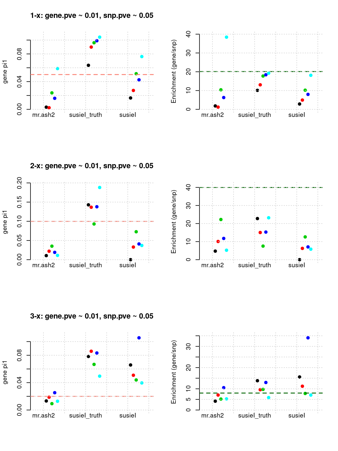

Version	Author	Date
c1c6bcc	simingz	2020-09-14
4d39fd6	simingz	2020-09-14

par(mfrow = c(1,3))
gpip_dist(susieIfs2[1:5], main = "1-x combined")
gpip_dist(susieIfs2[6:10], main = "2-x combined")
gpip_dist(susieIfs2[11:15], main = "3-x combined")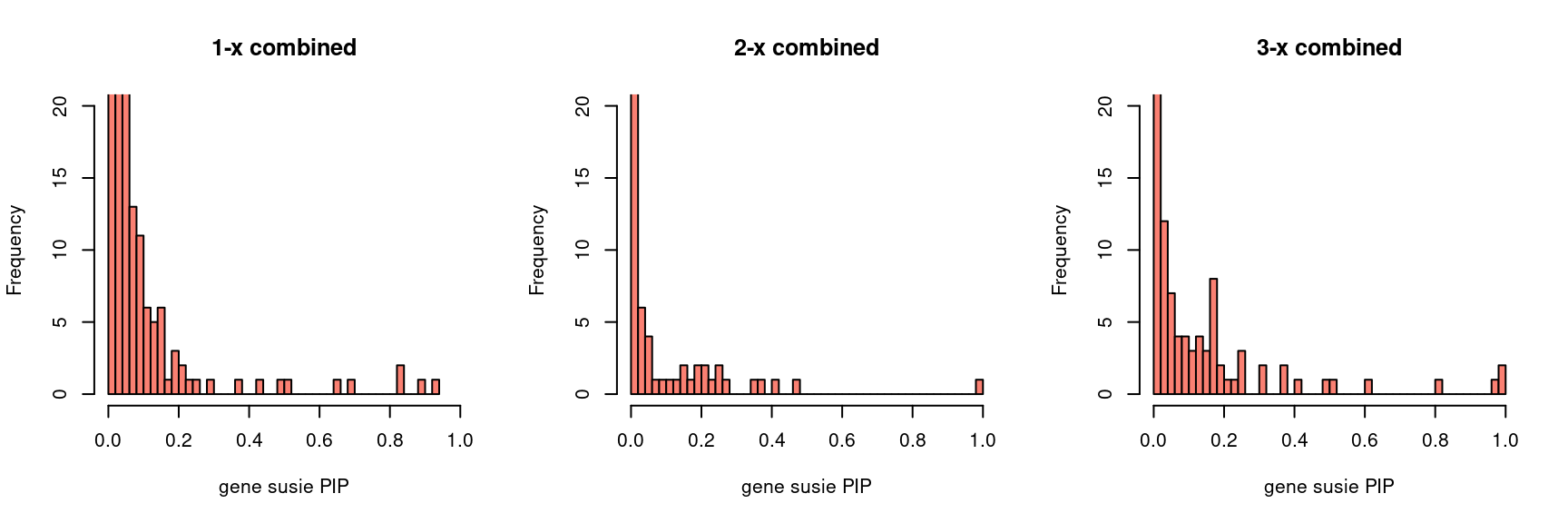

Regions: mrash gene+SNP (1)

Regions: We use regional PIP of both SNP and gene from mr.ash2s > 0.3.
Susie run parameters: L=2, initialize null_weight = 0, update null_weight in iterations. We initialize with prior for genes and SNPs as uniform. (We also tried initialize with prior for genes and SNPs as 0.05 and 2.5e-3, results are the same.)

tags <- paste(rep(1:4, each = 5), 1:5, sep = "-")
mr.ashfs <- paste0(mrashdir, "20200721-", tags, "-mr.ash2s.lassoes-es.param.txt")
susieIfs <- paste0(outputdir, "20200813-", tags, ".config6.susieIres.Rd")
susieIfs2 <- paste0(outputdir, "20200813-", tags, ".config6.susieI.txt")

df <- show_param(mrashfs, susieIfs, susieIfs2)
par(mfrow = c(4,2))
plot_param(df[1:5,], main = "1-x: gene.pve ~ 0.01, snp.pve ~ 0.05")
plot_param(df[6:10,], main = "2-x: gene.pve ~ 0.01, snp.pve ~ 0.05")
plot_param(df[11:15,], main = "3-x: gene.pve ~ 0.01, snp.pve ~ 0.05")
plot_param(df[16:20,], main = "4-x: gene.pve ~ 0.05, snp.pve ~ 0.05")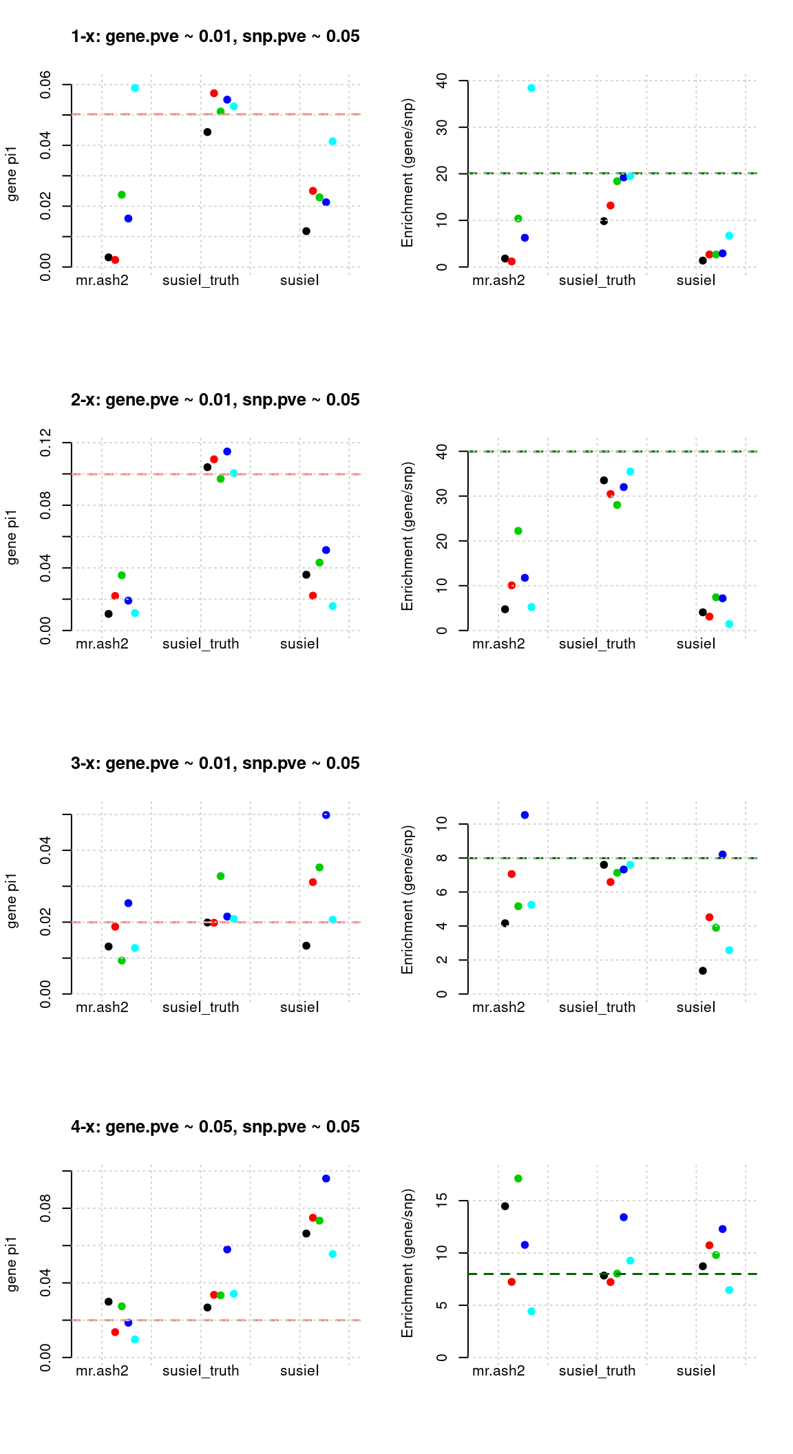

Version	Author	Date
c1c6bcc	simingz	2020-09-14
4d39fd6	simingz	2020-09-14

par(mfrow = c(1,4))
gpip_dist(susieIfs2[1:5], main = "1-x combined")
gpip_dist(susieIfs2[6:10], main = "2-x combined")
gpip_dist(susieIfs2[11:15], main = "3-x combined")
gpip_dist(susieIfs2[16:20], main = "4-x combined")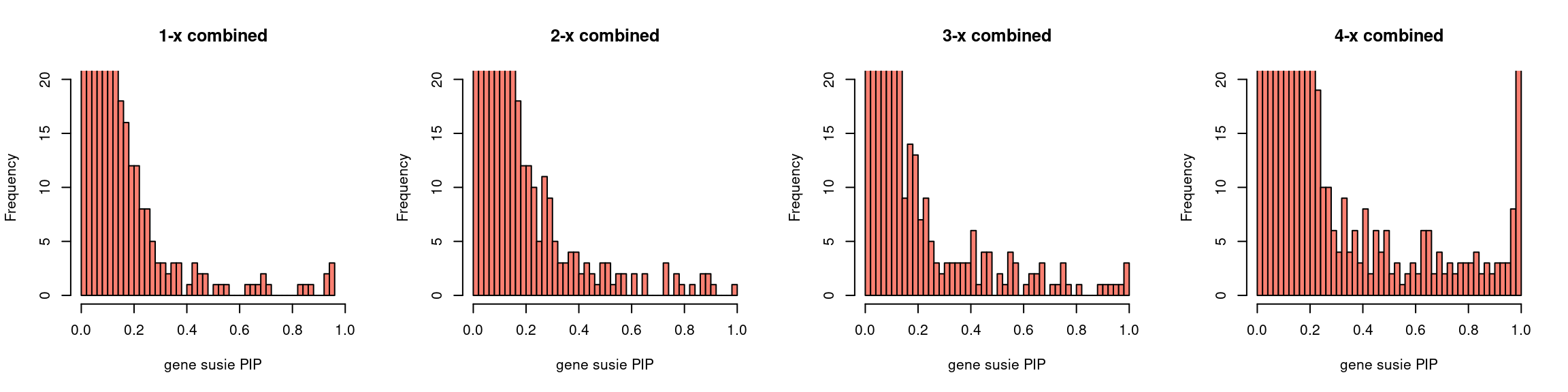

Regions: mrash gene+SNP (2)

Regions: We use regional PIP of both SNP and gene from mr.ash2s > 0.3.
Susie run parameters: L=2, null_weight = 0. Didn’t update null_weight in iterations. We initialize with prior for genes and SNPs as uniform.

tags <- paste(rep(1:4, each = 5), 1:5, sep = "-")
susieIfs <- paste0(outputdir, "20200813-", tags, ".config7.susieIres.Rd")
susieIfs2 <- paste0(outputdir, "20200813-", tags, ".config7.susieI.txt")

df <- show_param(mrashfs, susieIfs, susieIfs2)
par(mfrow = c(4,2))
plot_param(df[1:5,], main = "1-x: gene.pve ~ 0.01, snp.pve ~ 0.05")
plot_param(df[6:10,], main = "2-x: gene.pve ~ 0.01, snp.pve ~ 0.05")
plot_param(df[11:15,], main = "3-x: gene.pve ~ 0.01, snp.pve ~ 0.05")
plot_param(df[16:20,], main = "4-x: gene.pve ~ 0.05, snp.pve ~ 0.05")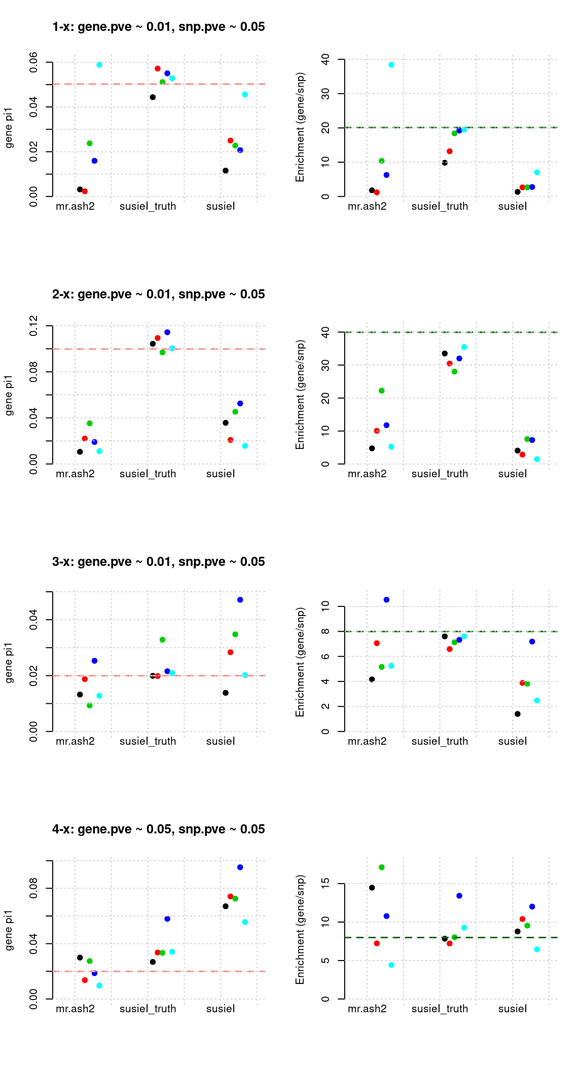

Version	Author	Date
c1c6bcc	simingz	2020-09-14
4d39fd6	simingz	2020-09-14

par(mfrow = c(1,4))
gpip_dist(susieIfs2[1:5], main = "1-x combined")
gpip_dist(susieIfs2[6:10], main = "2-x combined")
gpip_dist(susieIfs2[11:15], main = "3-x combined")
gpip_dist(susieIfs2[16:20], main = "4-x combined")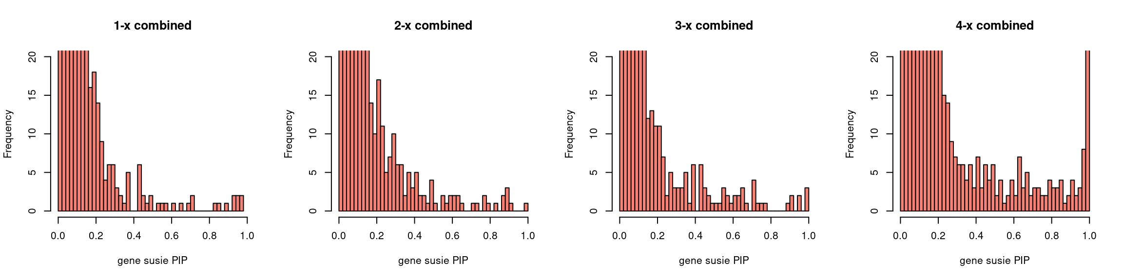

Regions: mrash gene only

Regions: We use regional sum of PIP for genes from mr.ash for genes only > 0.1.
Susie run parameters: L=2. Update null_weight in iterations. We initialize with prior for genes and SNPs as uniform, null_weight = 0.

tags <- paste(rep(1:4, each = 5), 1:5, sep = "-")
susieIfs <- paste0(outputdir, "20200813-", tags, ".config9.susieIres.Rd")
susieIfs2 <- paste0(outputdir, "20200813-", tags, ".config9.susieI.txt")

df <- show_param(mrashfs, susieIfs, susieIfs2)
par(mfrow = c(4,2))
plot_param(df[1:5,], main = "1-x: gene.pve ~ 0.01, snp.pve ~ 0.05")
plot_param(df[6:10,], main = "2-x: gene.pve ~ 0.01, snp.pve ~ 0.05")
plot_param(df[11:15,], main = "3-x: gene.pve ~ 0.01, snp.pve ~ 0.05")
plot_param(df[16:20,], main = "4-x: gene.pve ~ 0.05, snp.pve ~ 0.05")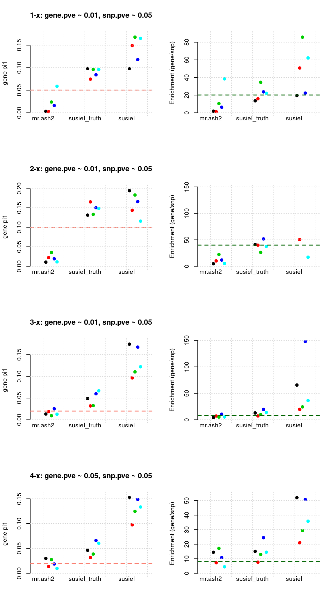

Version	Author	Date
c1c6bcc	simingz	2020-09-14
4d39fd6	simingz	2020-09-14

par(mfrow = c(1,4))
gpip_dist(susieIfs2[1:5], main = "1-x combined")
gpip_dist(susieIfs2[6:10], main = "2-x combined")
gpip_dist(susieIfs2[11:15], main = "3-x combined")
gpip_dist(susieIfs2[16:20], main = "4-x combined")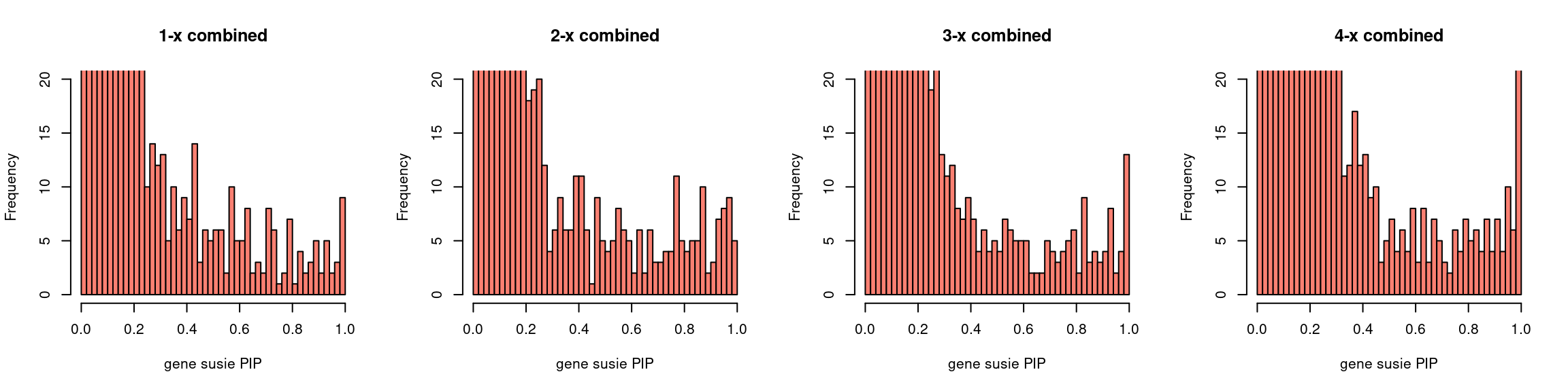

Regions: TWAS gene only

Regions: We use regional min p value for genes from twas for genes only, requiring this p value in top 5%.
Susie run parameters: L=2. Update null_weight in iterations. We initialize with prior for genes and SNPs as uniform, null_weight = 0.

tags <- paste(rep(1:4, each = 5), 1:5, sep = "-")
susieIfs <- paste0(outputdir, "20200813-", tags, ".config10.susieIres.Rd")
susieIfs2 <- paste0(outputdir, "20200813-", tags, ".config10.susieI.txt")

df <- show_param(mrashfs, susieIfs, susieIfs2)
par(mfrow = c(4,2))
plot_param(df[1:5,], main = "1-x: gene.pve ~ 0.01, snp.pve ~ 0.05")
plot_param(df[6:10,], main = "2-x: gene.pve ~ 0.01, snp.pve ~ 0.05")
plot_param(df[11:15,], main = "3-x: gene.pve ~ 0.01, snp.pve ~ 0.05")
plot_param(df[16:20,], main = "4-x: gene.pve ~ 0.05, snp.pve ~ 0.05")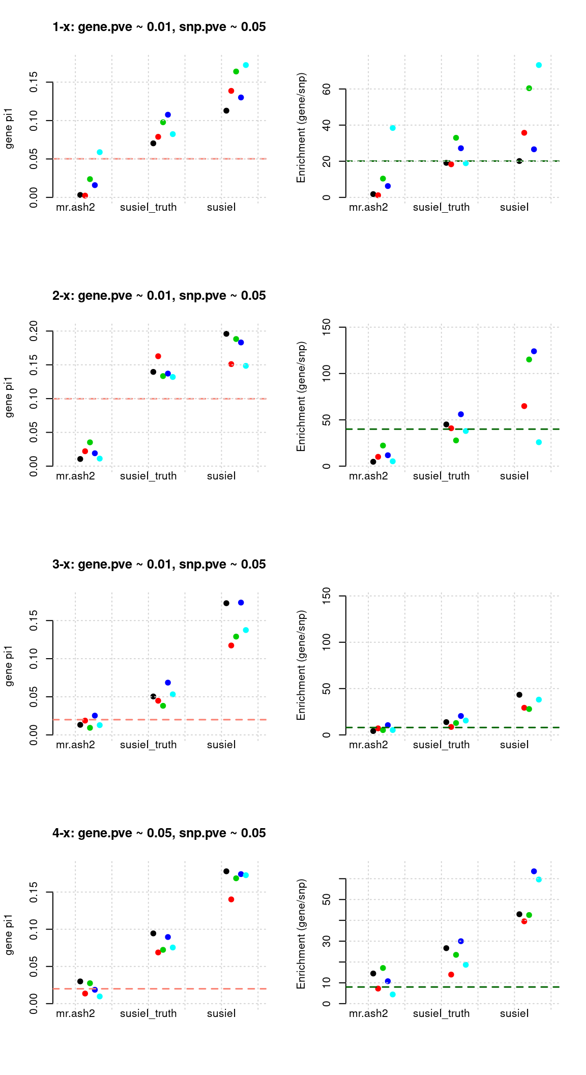

Version	Author	Date
c1c6bcc	simingz	2020-09-14
4d39fd6	simingz	2020-09-14

par(mfrow = c(1,4))
gpip_dist(susieIfs2[1:5], main = "1-x combined")
gpip_dist(susieIfs2[6:10], main = "2-x combined")
gpip_dist(susieIfs2[11:15], main = "3-x combined")
gpip_dist(susieIfs2[16:20], main = "4-x combined")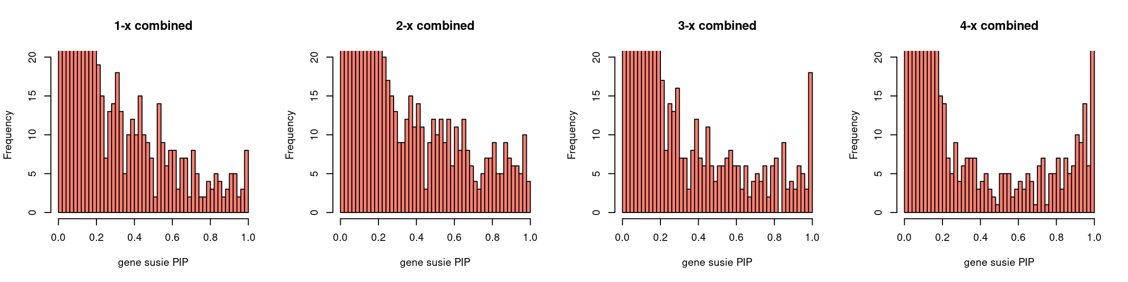

Regions: TWAS gene+SNP top

Regions: We use regional min p value for genes or SNPs from twas for genes and snps, requiring this p value in top 5% for genes or 1% for SNPs.
Susie run parameters: L=2. Update null_weight in iterations. We initialize with prior for genes and SNPs as uniform, null_weight = 0.

tags <- paste(rep(1:4, each = 5), 1:5, sep = "-")
susieIfs <- paste0(outputdir, "20200813-", tags, ".config11.susieIres.Rd")
susieIfs2 <- paste0(outputdir, "20200813-", tags, ".config11.susieI.txt")

df <- show_param(mrashfs, susieIfs, susieIfs2)
par(mfrow = c(4,2))
plot_param(df[1:5,], main = "1-x: gene.pve ~ 0.01, snp.pve ~ 0.05")
plot_param(df[6:10,], main = "2-x: gene.pve ~ 0.01, snp.pve ~ 0.05")
plot_param(df[11:15,], main = "3-x: gene.pve ~ 0.01, snp.pve ~ 0.05")
plot_param(df[16:20,], main = "4-x: gene.pve ~ 0.05, snp.pve ~ 0.05")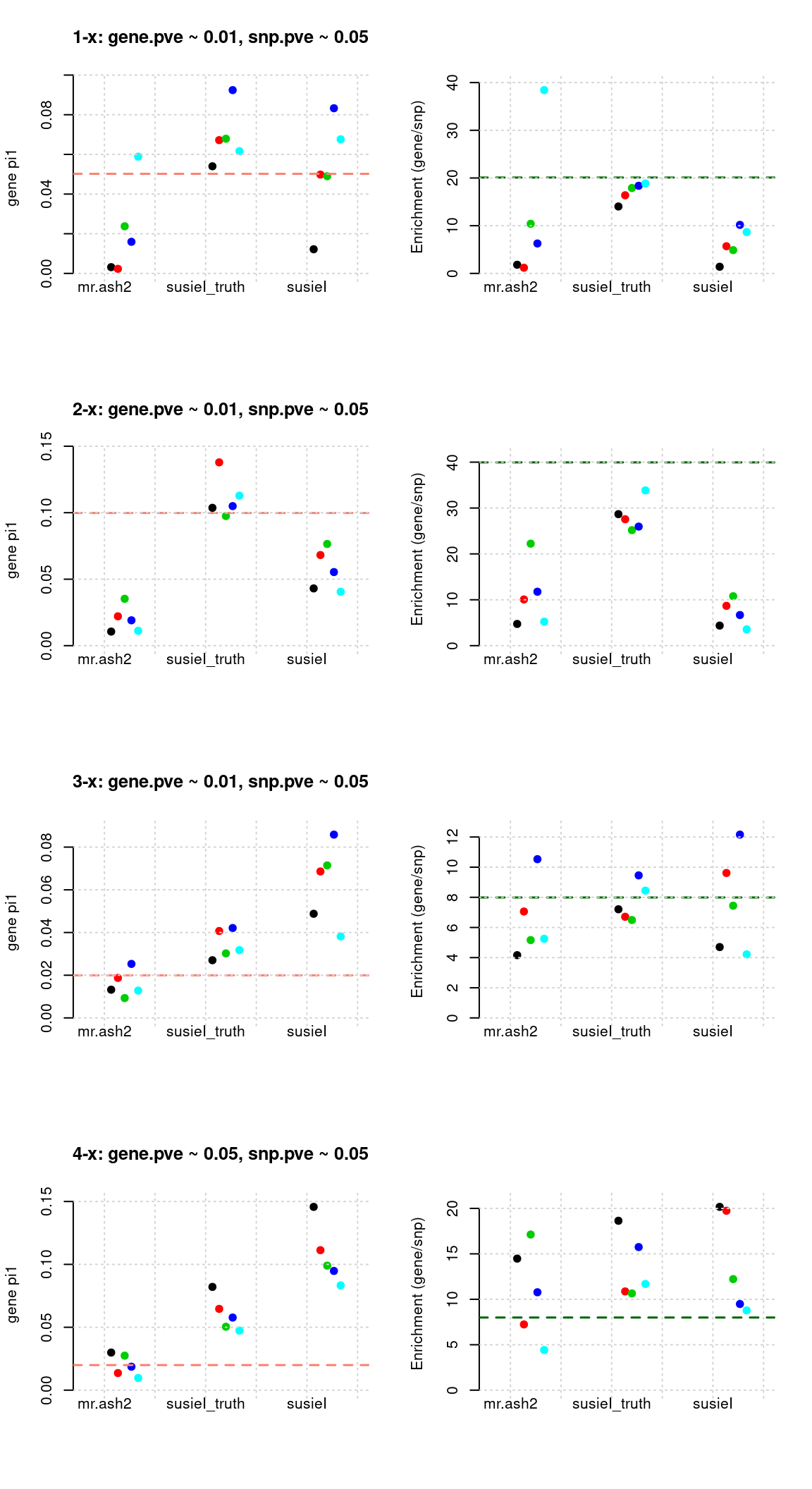

Version	Author	Date
c1c6bcc	simingz	2020-09-14
4d39fd6	simingz	2020-09-14

par(mfrow = c(1,4))
gpip_dist(susieIfs2[1:5], main = "1-x combined")
gpip_dist(susieIfs2[6:10], main = "2-x combined")
gpip_dist(susieIfs2[11:15], main = "3-x combined")
gpip_dist(susieIfs2[16:20], main = "4-x combined")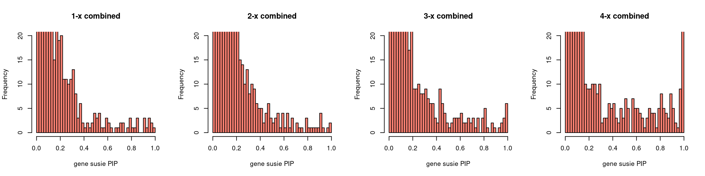

Regions: TWAS gene+SNP BF

Regions: get BF for both genes and SNPs. regional TWAS BF > 2

tags <- paste(rep(1:4, each = 5), 1:5, sep = "-")
mr.ashfs <- paste0(mrashdir, "20200721-", tags, "-mr.ash2s.lassoes-es.param.txt")
susieIfs <- paste0(outputdir, "20200813-", tags, ".config12.susieIres.Rd")
susieIfs2 <- paste0(outputdir, "20200813-", tags, ".config12.susieI.txt")

df <- show_param(mrashfs, susieIfs, susieIfs2)
par(mfrow = c(4,2))
plot_param(df[1:5,], main = "1-x: gene.pve ~ 0.01, snp.pve ~ 0.05")
plot_param(df[6:10,], main = "2-x: gene.pve ~ 0.01, snp.pve ~ 0.05")
plot_param(df[11:15,], main = "3-x: gene.pve ~ 0.01, snp.pve ~ 0.05")
plot_param(df[16:20,], main = "4-x: gene.pve ~ 0.05, snp.pve ~ 0.05")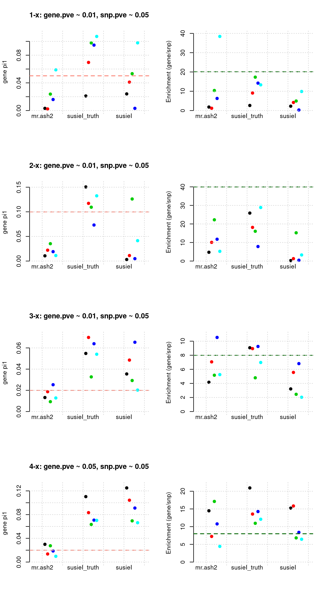

Version	Author	Date
34b9ed3	simingz	2020-09-18

par(mfrow = c(1,4))
gpip_dist(susieIfs2[1:5], main = "1-x combined")
gpip_dist(susieIfs2[6:10], main = "2-x combined")
gpip_dist(susieIfs2[11:15], main = "3-x combined")
gpip_dist(susieIfs2[16:20], main = "4-x combined")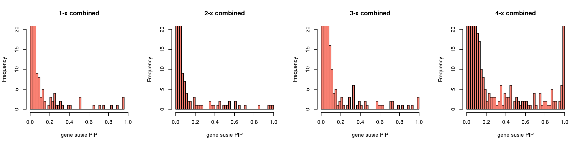

Regions: TWAS gene+SNP FDR

Regions: put gene and SNP pvalues together and get FDR. Seelect regions with minimum FDR < 0.05.

tags <- paste(rep(1:4, each = 5), 1:5, sep = "-")
mr.ashfs <- paste0(mrashdir, "20200721-", tags, "-mr.ash2s.lassoes-es.param.txt")
susieIfs <- paste0(outputdir, "20200813-", tags, ".config13.susieIres.Rd")
susieIfs2 <- paste0(outputdir, "20200813-", tags, ".config13.susieI.txt")

df <- show_param(mrashfs, susieIfs, susieIfs2)
par(mfrow = c(4,2))
plot_param(df[1:5,], main = "1-x: gene.pve ~ 0.01, snp.pve ~ 0.05")
plot_param(df[6:10,], main = "2-x: gene.pve ~ 0.01, snp.pve ~ 0.05")
plot_param(df[11:15,], main = "3-x: gene.pve ~ 0.01, snp.pve ~ 0.05")
plot_param(df[16:20,], main = "4-x: gene.pve ~ 0.05, snp.pve ~ 0.05")

par(mfrow = c(1,4))
gpip_dist(susieIfs2[1:5], main = "1-x combined")
gpip_dist(susieIfs2[6:10], main = "2-x combined")
gpip_dist(susieIfs2[11:15], main = "3-x combined")
gpip_dist(susieIfs2[16:20], main = "4-x combined")

Regions: all (1)

Regions: All regions.
Susie run parameters: L=2. initialize with null_weight = 0 and update null_weight based on last iteration results. We initialize with prior for genes and SNPs as uniform.

mr.ashfs <- paste0(mrashdir, "20200721-", tags, "-mr.ash2s.lassoes-es.param.txt")
susieIfs <- paste0(outputdir, "20200813-", tags, ".config2.susieIres.Rd")
susieIfs2 <- paste0(outputdir, "20200813-", tags, ".config2.susieI.txt")

df <- show_param(mrashfs, susieIfs, susieIfs2)
par(mfrow = c(4,2))
plot_param(df[1:5,], main = "1-x: gene.pve ~ 0.01, snp.pve ~ 0.05")
plot_param(df[6:10,], main = "2-x: gene.pve ~ 0.01, snp.pve ~ 0.05")
plot_param(df[11:15,], main = "3-x: gene.pve ~ 0.01, snp.pve ~ 0.05")
plot_param(df[16:20,], main = "4-x: gene.pve ~ 0.05, snp.pve ~ 0.05")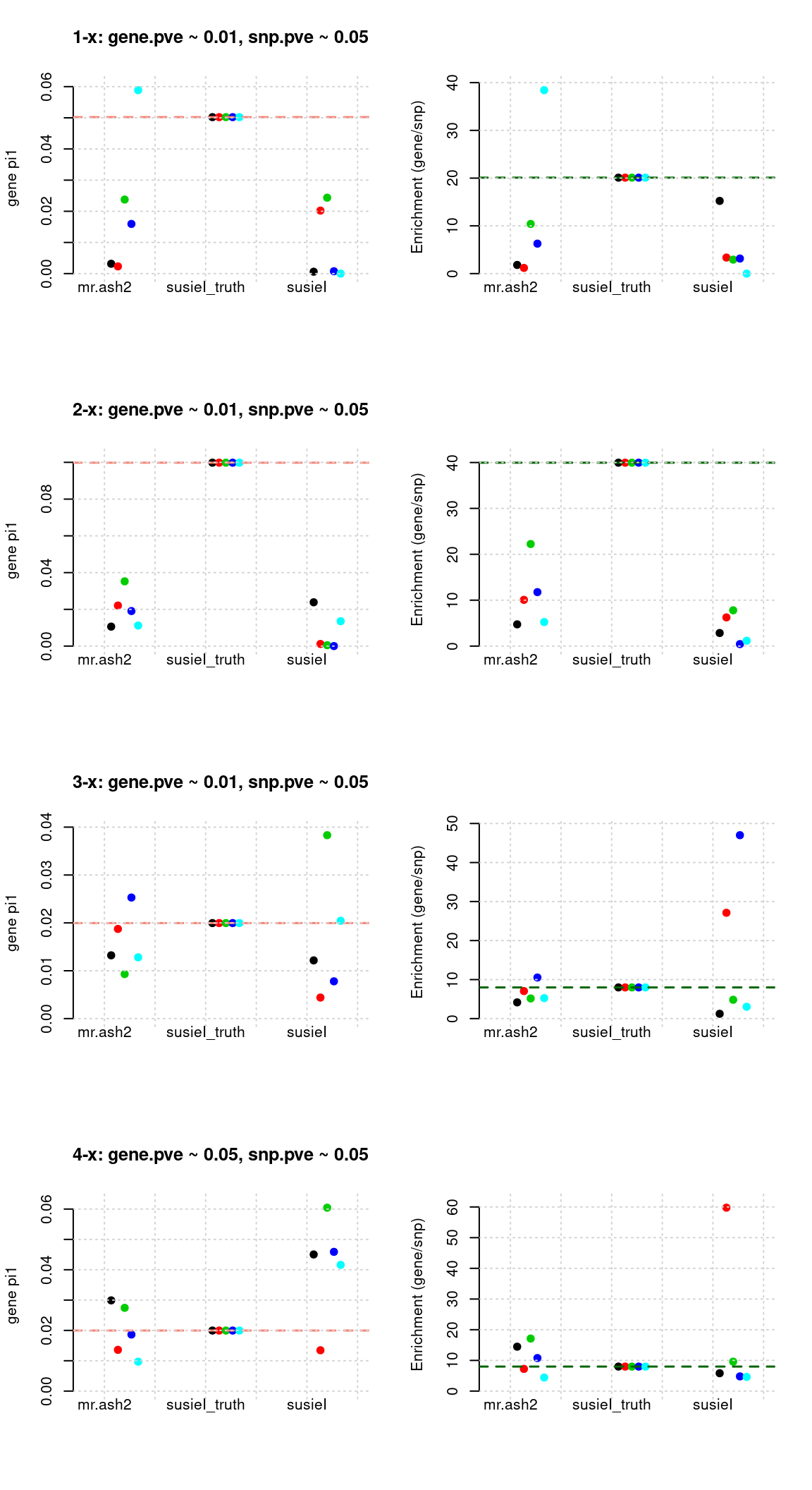

Version	Author	Date
c1c6bcc	simingz	2020-09-14
4d39fd6	simingz	2020-09-14

par(mfrow = c(1,4))
gpip_dist(susieIfs2[1:5], main = "1-x combined")
gpip_dist(susieIfs2[6:10], main = "2-x combined")
gpip_dist(susieIfs2[11:15], main = "3-x combined")
gpip_dist(susieIfs2[16:20], main = "4-x combined")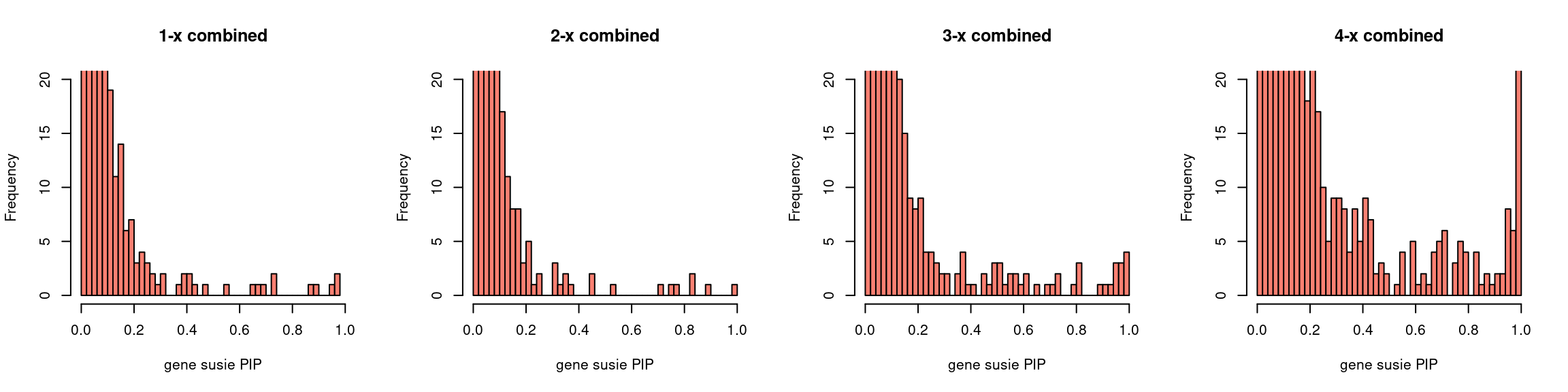

Regions: all (2)

Regions: All regions.
Susie run parameters: L=1. Did not update null_weight in each iteration. We initialize with prior for genes and SNPs as uniform.

mr.ashfs <- paste0(mrashdir, "20200721-", tags, "-mr.ash2s.lassoes-es.param.txt")
susieIfs <- paste0(outputdir, "20200813-", tags, ".config3.susieIres.Rd")
susieIfs2 <- paste0(outputdir, "20200813-", tags, ".config3.susieI.txt")

df <- show_param(mrashfs, susieIfs, susieIfs2)
par(mfrow = c(4,2))
plot_param(df[1:5,], main = "1-x: gene.pve ~ 0.01, snp.pve ~ 0.05")
plot_param(df[6:10,], main = "2-x: gene.pve ~ 0.01, snp.pve ~ 0.05")
plot_param(df[11:15,], main = "3-x: gene.pve ~ 0.01, snp.pve ~ 0.05")
plot_param(df[16:20,], main = "4-x: gene.pve ~ 0.05, snp.pve ~ 0.05")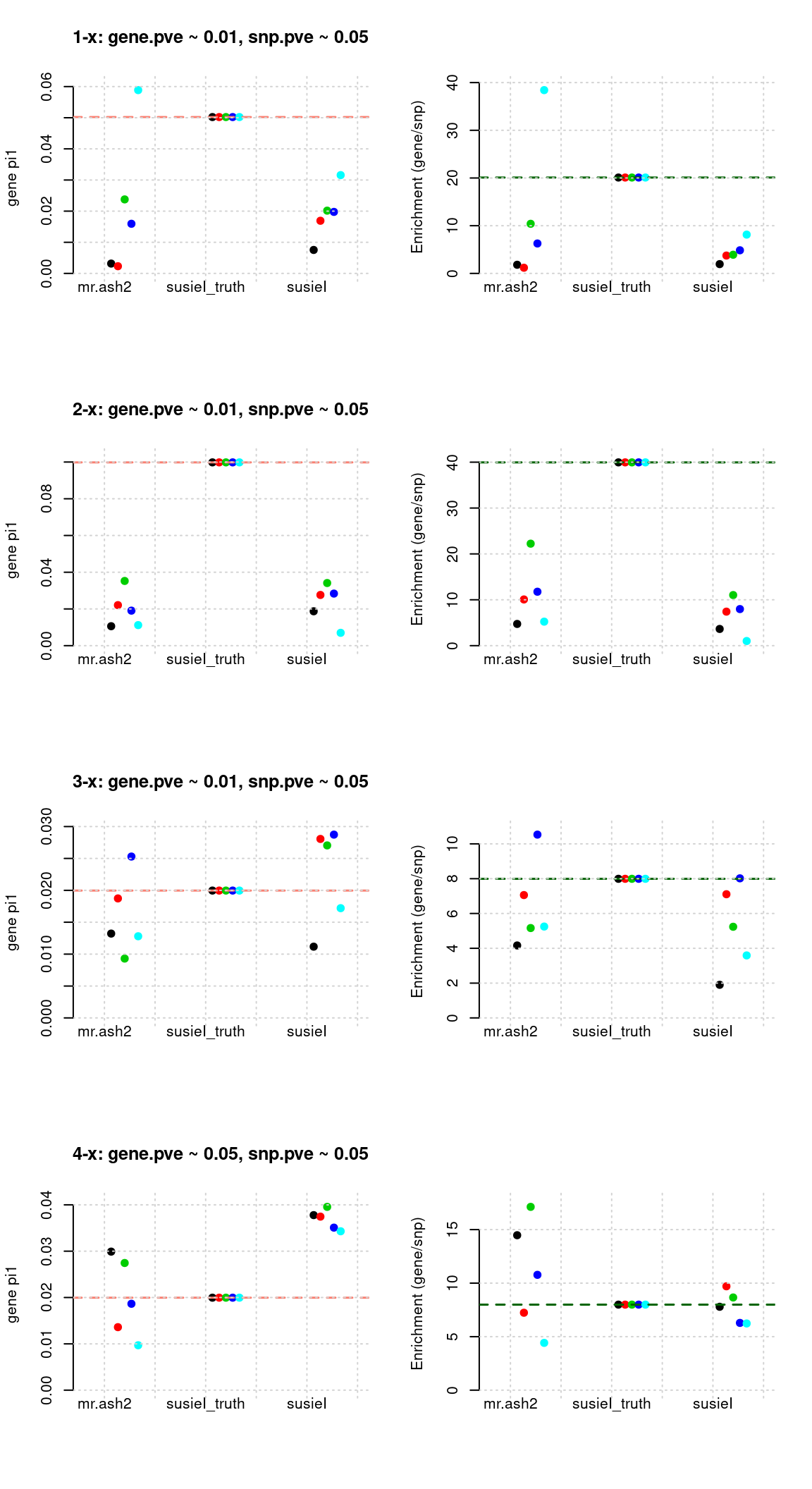

Version	Author	Date
c1c6bcc	simingz	2020-09-14
4d39fd6	simingz	2020-09-14

par(mfrow = c(1,4))
gpip_dist(susieIfs2[1:5], main = "1-x combined")
gpip_dist(susieIfs2[6:10], main = "2-x combined")
gpip_dist(susieIfs2[11:15], main = "3-x combined")
gpip_dist(susieIfs2[16:20], main = "4-x combined")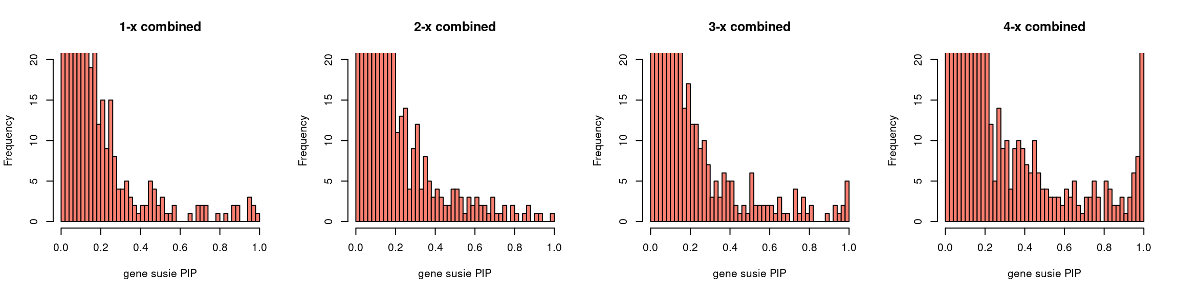

Regions: all (others)

Susie run parameters: L=1. initialize with null_weight = 0 and update null_weight based on last iteration results. We initialize with prior for genes and SNPs as uniform. The prior for genes is underestimated for low power settings (1-x, 2-x), many converged to close to 0, for high power settings it is better.
Susie run parameters: L=5. initialize with null_weight = 0 and update null_weight based on last iteration results. The prior for gene estimation is fine for all runs, however prior for SNPs overestimated about 10 times.
We have tried different initiation strategies, but the results remain the same.

sessionInfo()

R version 3.5.1 (2018-07-02)
Platform: x86_64-pc-linux-gnu (64-bit)
Running under: Scientific Linux 7.4 (Nitrogen)

Matrix products: default
BLAS/LAPACK: /software/openblas-0.2.19-el7-x86_64/lib/libopenblas_haswellp-r0.2.19.so

locale:
 [1] LC_CTYPE=en_US.UTF-8       LC_NUMERIC=C              
 [3] LC_TIME=en_US.UTF-8        LC_COLLATE=en_US.UTF-8    
 [5] LC_MONETARY=en_US.UTF-8    LC_MESSAGES=en_US.UTF-8   
 [7] LC_PAPER=en_US.UTF-8       LC_NAME=C                 
 [9] LC_ADDRESS=C               LC_TELEPHONE=C            
[11] LC_MEASUREMENT=en_US.UTF-8 LC_IDENTIFICATION=C       

attached base packages:
[1] stats     graphics  grDevices utils     datasets  methods   base     

other attached packages:
[1] kableExtra_1.2.1    stringr_1.4.0       plyr_1.8.6         
[4] tidyr_0.8.3         plotly_4.9.2.9000   ggplot2_3.3.1      
[7] data.table_1.12.7   mr.ash.alpha_0.1-34

loaded via a namespace (and not attached):
 [1] tidyselect_1.1.0  purrr_0.3.4       lattice_0.20-38  
 [4] colorspace_1.3-2  vctrs_0.3.1       generics_0.0.2   
 [7] htmltools_0.3.6   viridisLite_0.3.0 yaml_2.2.0       
[10] rlang_0.4.6       later_0.7.5       pillar_1.4.4     
[13] glue_1.4.1        withr_2.1.2       lifecycle_0.2.0  
[16] munsell_0.5.0     gtable_0.2.0      workflowr_1.6.2  
[19] rvest_0.3.2       htmlwidgets_1.3   evaluate_0.12    
[22] knitr_1.20        httpuv_1.4.5      Rcpp_1.0.4.6     
[25] promises_1.0.1    scales_1.0.0      backports_1.1.2  
[28] webshot_0.5.1     jsonlite_1.6.1    fs_1.3.1         
[31] digest_0.6.25     stringi_1.3.1     dplyr_1.0.0      
[34] grid_3.5.1        rprojroot_1.3-2   here_0.1         
[37] tools_3.5.1       magrittr_1.5      lazyeval_0.2.1   
[40] tibble_3.0.1      crayon_1.3.4      whisker_0.3-2    
[43] pkgconfig_2.0.2   ellipsis_0.3.1    Matrix_1.2-15    
[46] xml2_1.2.0        rmarkdown_1.10    httr_1.4.1       
[49] rstudioapi_0.11   R6_2.3.0          git2r_0.26.1     
[52] compiler_3.5.1

Test susieI using chr17 to 22