Mr.ash2 parameter estimation

NULL; expr-snp; expr-snp
NULL; snp-expr; expr-snp
lasso; expr-snp; expr-snp
lasso; expr-snp; snp-expr

Regional mr.ash2s PIP overview

PIP calibration

NULL; expr-snp; expr-snp
Lasso; expr-snp; expr-snp

PIP scatter plot

NULL; expr-snp; expr-snp
NULL; snp-expr; expr-snp
lasso; expr-snp; expr-snp
lasso; expr-snp; snp-expr

ROC curve

NULL; expr-snp; expr-snp
NULL; snp-expr; expr-snp
lasso; expr-snp; expr-snp
lasso; expr-snp; snp-expr

PIP vs p value

NULL; expr-snp; expr-snp

Last updated: 2020-08-10

Checks: 7 0

Knit directory: causal-TWAS/

This reproducible R Markdown analysis was created with workflowr (version 1.6.2). The Checks tab describes the reproducibility checks that were applied when the results were created. The Past versions tab lists the development history.

R Markdown file: up-to-date

Great! Since the R Markdown file has been committed to the Git repository, you know the exact version of the code that produced these results.

Environment: empty

Great job! The global environment was empty. Objects defined in the global environment can affect the analysis in your R Markdown file in unknown ways. For reproduciblity it’s best to always run the code in an empty environment.

Seed: set.seed(20191103)

The command set.seed(20191103) was run prior to running the code in the R Markdown file. Setting a seed ensures that any results that rely on randomness, e.g. subsampling or permutations, are reproducible.

Session information: recorded

Great job! Recording the operating system, R version, and package versions is critical for reproducibility.

Cache: none

Nice! There were no cached chunks for this analysis, so you can be confident that you successfully produced the results during this run.

File paths: relative

Great job! Using relative paths to the files within your workflowr project makes it easier to run your code on other machines.

Repository version: 2903ad5

Great! You are using Git for version control. Tracking code development and connecting the code version to the results is critical for reproducibility.

The results in this page were generated with repository version 2903ad5. See the Past versions tab to see a history of the changes made to the R Markdown and HTML files.

Note that you need to be careful to ensure that all relevant files for the analysis have been committed to Git prior to generating the results (you can use wflow_publish or wflow_git_commit). workflowr only checks the R Markdown file, but you know if there are other scripts or data files that it depends on. Below is the status of the Git repository when the results were generated:


Ignored files:
    Ignored:    .Rhistory
    Ignored:    .Rproj.user/
    Ignored:    code/workflow/.ipynb_checkpoints/
    Ignored:    data/

Unstaged changes:
    Modified:   analysis/summarize_twas_plots.R
    Modified:   code/run_test_mr.ash2s.R

Note that any generated files, e.g. HTML, png, CSS, etc., are not included in this status report because it is ok for generated content to have uncommitted changes.

These are the previous versions of the repository in which changes were made to the R Markdown (analysis/simulation-multi-ukbchr22-gtex.adipose2.Rmd) and HTML (docs/simulation-multi-ukbchr22-gtex.adipose2.html) files. If you’ve configured a remote Git repository (see ?wflow_git_remote), click on the hyperlinks in the table below to view the files as they were in that past version.

File	Version	Author	Date	Message
Rmd	9783727	simingz	2020-08-06	susie names
html	9783727	simingz	2020-08-06	susie names
Rmd	2216650	simingz	2020-08-06	Remove ignored files
html	2216650	simingz	2020-08-06	Remove ignored files
Rmd	958f794	simingz	2020-08-05	move code- plot functions
html	958f794	simingz	2020-08-05	move code- plot functions
Rmd	86e42c2	simingz	2020-08-04	website hide code
html	86e42c2	simingz	2020-08-04	website hide code
Rmd	f6ea15c	simingz	2020-08-04	change sa2 grid
html	f6ea15c	simingz	2020-08-04	change sa2 grid
Rmd	89b90ad	simingz	2020-07-24	chr17:22
html	89b90ad	simingz	2020-07-24	chr17:22

Run simulation 9 times for ukb chr 22.

library(mr.ash.alpha)
library(data.table)
suppressMessages({library(plotly)})
library(tidyr)
library(plyr)
library(stringr)
library(kableExtra)
source("analysis/summarize_twas_plots.R")

simdatadir <- "~/causalTWAS/simulations/simulation_ashtest_20200616/"
outputdir <- "~/causalTWAS/simulations/simulation_ashtest_20200616/"
susiedir <- "~/causalTWAS/simulations/simulation_susietest_20200616/"
tags <- paste0('20200616-8-', 1:9)
tagglob <- '20200616-8-*'
tagextr <- '20200616-8-\\d+'
tag2s <- c('zeroes-es', 'zerose-es', 'lassoes-es','lassoes-se')

Mr.ash2 parameter estimation

Results for 9 simulations runs, using different initialize and update strategy

show_param <- function(tags, tag2){
  f <- lapply(tags, get_files, tag2 = tag2)
  parf <- lapply(f, '[[', "par")
  param <- do.call(rbind, lapply(parf, function(x) t(read.table(x))[2:1,]))
  truth <- param[1:(nrow(param)/2)*2-1,]
  est <- param[1:(nrow(param)/2)*2,]
  outdt <- matrix(0, ncol = 2*ncol(param), nrow = nrow(param)/2)
  outdt[,c(1,3,5,7)] <- truth
  outdt[,c(2,4,6,8)] <- est
  outdt <-cbind(1:nrow(outdt),outdt)
  colnames(outdt) <- c("Simulation#", paste0(rep(c("Truth","Est."),4)))
  knitr::kable(outdt) %>%
  kable_styling("striped") %>%
  add_header_above(c(" " = 1, "Gene.pi1" = 2, "Gene.PVE" = 2, "SNP.pi1" = 2, "SNP.PVE" =2))
}

NULL; expr-snp; expr-snp

show_param(tags = tags, tag2 = tag2s[1])

	Gene.pi1		Gene.PVE		SNP.pi1		SNP.PVE
Simulation#	Truth	Est.	Truth	Est.	Truth	Est.	Truth	Est.
1	0.0209205	0.0222753	0.0060041	0.0257131	0.0002559	0.0002721	0.0611847	0.0476191
2	0.0209205	0.0293598	0.0125625	0.0148927	0.0002559	0.0001422	0.0623990	0.0565124
3	0.0209205	0.0248155	0.0143559	0.0270832	0.0002559	0.0002346	0.0651471	0.0538022
4	0.0209205	0.0392044	0.0095282	0.0134942	0.0002559	0.0002832	0.0504149	0.0285669
5	0.0209205	0.0096836	0.0076604	0.0117105	0.0002559	0.0002105	0.0411680	0.0474628
6	0.0209205	0.0327729	0.0088879	0.0160215	0.0002559	0.0001661	0.0465910	0.0392070
7	0.0209205	0.0464974	0.0075311	0.0141466	0.0002559	0.0001922	0.0742512	0.0739697
8	0.0209205	0.0183843	0.0095491	0.0170822	0.0002559	0.0002301	0.0748342	0.0774682
9	0.0209205	0.0327868	0.0124448	0.0146459	0.0002559	0.0001889	0.0395446	0.0461935

NULL; snp-expr; expr-snp

show_param(tags = tags, tag2 = tag2s[2])

	Gene.pi1		Gene.PVE		SNP.pi1		SNP.PVE
Simulation#	Truth	Est.	Truth	Est.	Truth	Est.	Truth	Est.
1	0.0209205	0.0222753	0.0060041	0.0257131	0.0002559	0.0002721	0.0611847	0.0476191
2	0.0209205	0.0293589	0.0125625	0.0148945	0.0002559	0.0001422	0.0623990	0.0565125
3	0.0209205	0.0248155	0.0143559	0.0270832	0.0002559	0.0002346	0.0651471	0.0538022
4	0.0209205	0.0392026	0.0095282	0.0134994	0.0002559	0.0002832	0.0504149	0.0285687
5	0.0209205	0.0096836	0.0076604	0.0117105	0.0002559	0.0002105	0.0411680	0.0474627
6	0.0209205	0.0327729	0.0088879	0.0160215	0.0002559	0.0001661	0.0465910	0.0392070
7	0.0209205	0.0464974	0.0075311	0.0141466	0.0002559	0.0001922	0.0742512	0.0739697
8	0.0209205	0.0183844	0.0095491	0.0170820	0.0002559	0.0002301	0.0748342	0.0774678
9	0.0209205	0.0327868	0.0124448	0.0146459	0.0002559	0.0001889	0.0395446	0.0461936

lasso; expr-snp; expr-snp

show_param(tags = tags, tag2 = tag2s[3])

	Gene.pi1		Gene.PVE		SNP.pi1		SNP.PVE
Simulation#	Truth	Est.	Truth	Est.	Truth	Est.	Truth	Est.
1	0.0209205	0.0069797	0.0060041	0.0020441	0.0002559	0.0002275	0.0611847	0.0614937
2	0.0209205	0.0207931	0.0125625	0.0147445	0.0002559	0.0001572	0.0623990	0.0622327
3	0.0209205	0.0114924	0.0143559	0.0140703	0.0002559	0.0002667	0.0651471	0.0683366
4	0.0209205	0.0136536	0.0095282	0.0040695	0.0002559	0.0003125	0.0504149	0.0504142
5	0.0209205	0.0091555	0.0076604	0.0111420	0.0002559	0.0002774	0.0411680	0.0279415
6	0.0209205	0.0113293	0.0088879	0.0123651	0.0002559	0.0001963	0.0465910	0.0511911
7	0.0209205	0.0122711	0.0075311	0.0120373	0.0002559	0.0002557	0.0742512	0.0965410
8	0.0209205	0.0101661	0.0095491	0.0119478	0.0002559	0.0002181	0.0748342	0.0838292
9	0.0209205	0.0195901	0.0124448	0.0075159	0.0002559	0.0002253	0.0395446	0.0610403

lasso; expr-snp; snp-expr

show_param(tags = tags, tag2 = tag2s[4])

	Gene.pi1		Gene.PVE		SNP.pi1		SNP.PVE
Simulation#	Truth	Est.	Truth	Est.	Truth	Est.	Truth	Est.
1	0.0209205	0.0069853	0.0060041	0.0020446	0.0002559	0.0002259	0.0611847	0.0621952
2	0.0209205	0.0212120	0.0125625	0.0139487	0.0002559	0.0001571	0.0623990	0.0622386
3	0.0209205	0.0115027	0.0143559	0.0140764	0.0002559	0.0002651	0.0651471	0.0691414
4	0.0209205	0.0136857	0.0095282	0.0040785	0.0002559	0.0003073	0.0504149	0.0534981
5	0.0209205	0.0092058	0.0076604	0.0110433	0.0002559	0.0002779	0.0411680	0.0277027
6	0.0209205	0.0116320	0.0088879	0.0118495	0.0002559	0.0001973	0.0465910	0.0507534
7	0.0209205	0.0127229	0.0075311	0.0111653	0.0002559	0.0002554	0.0742512	0.0966526
8	0.0209205	0.0102499	0.0095491	0.0117384	0.0002559	0.0002180	0.0748342	0.0838319
9	0.0209205	0.0197915	0.0124448	0.0070771	0.0002559	0.0002242	0.0395446	0.0616208

Regional mr.ash2s PIP overview

Take simulation 1 (NULL; expr-snp; expr-snp) as examples. We use region size 500kb and PIP cut off at 0.5 for SUSIE.

f <- get_files(tag= tags[1], tag2 = tag2s[1])
a <- read.table(f[["rpip"]], header = T)
par(mar=c(5, 4, 4, 6) + 0.1)
with(a, plot(p0, rPIP, col ='salmon', xlab = "position", ylab= "Sum of PIP", type = 'h', lwd = 2))
par(new = T)
with(a, plot(p0, nCausal, pch =19, col = "darkgreen",axes = FALSE, bty = "n", xlab = "", ylab = ""))
axis(side = 4)
mtext(side = 4, line = 3, 'No. causal signals')
legend("topleft",
       legend=c("Mr.ASH PIP", "# Causal"),
       lty=c(1,0), pch=c(NA, 19), col=c("salmon", "darkgreen"))
grid()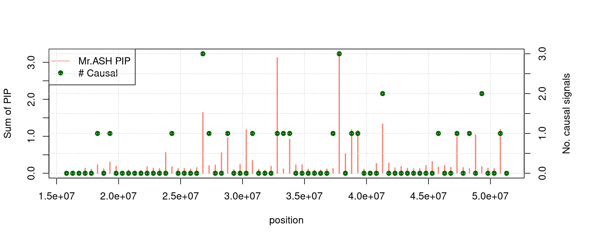

Version	Author	Date
f6ea15c	simingz	2020-08-04
89b90ad	simingz	2020-07-24

PIP calibration

We run 100 simulations and combine results.

NULL; expr-snp; expr-snp

tag2 = "zeroes-es"
tags_ext <- Reduce(intersect, get_tags(tagglob, tagextr, tag2 = tag2)['gsusie'])
res <- caliPIP_plot(tags = tags_ext, tag2 = tag2)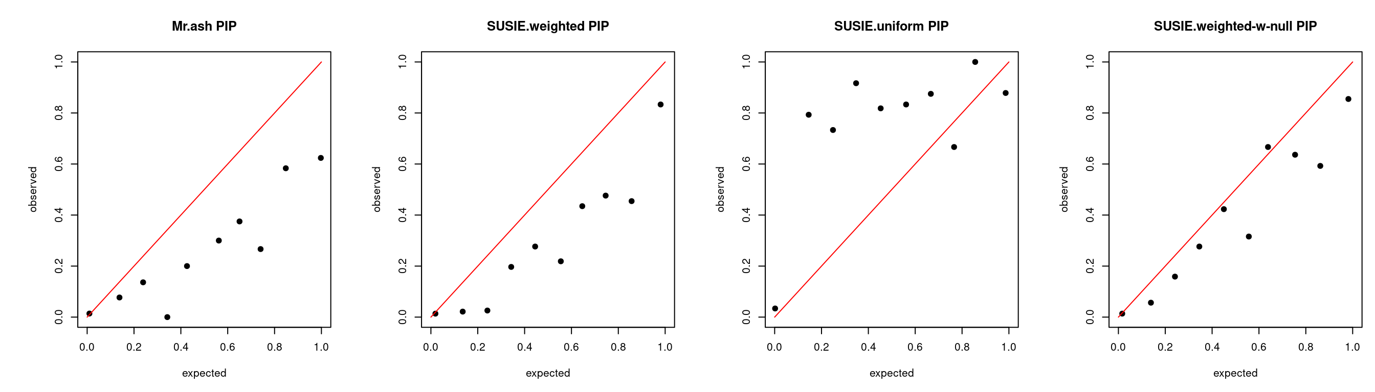

Version	Author	Date
9783727	simingz	2020-08-06
f6ea15c	simingz	2020-08-04

caliFDR_plot(tags = tags_ext, tag2 = tag2)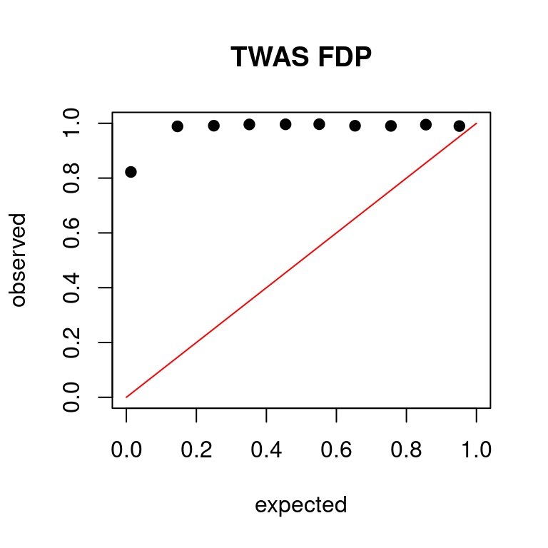

Version	Author	Date
f6ea15c	simingz	2020-08-04

FDR at bonferroni corrected p = 0.05:  0.71278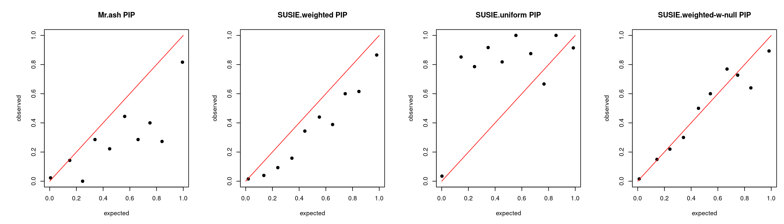

Lasso; expr-snp; expr-snp

caliPIP_plot(tags = tags_ext, tag2 = "lassoes-es")

Version	Author	Date
9783727	simingz	2020-08-06
f6ea15c	simingz	2020-08-04

caliFDR_plot(tags = tags_ext, tag2 = "lassoes-es")

Version	Author	Date
f6ea15c	simingz	2020-08-04

FDR at bonferroni corrected p = 0.05:  0.7059621

PIP scatter plot

mr.ash2s PIP vs. susie PIP.

NULL; expr-snp; expr-snp

scatter_plot_PIP(tags = tags, tag2 = tag2s[1])

NULL; snp-expr; expr-snp

scatter_plot_PIP(tags = tags, tag2 = tag2s[2])

lasso; expr-snp; expr-snp

scatter_plot_PIP(tags = tags, tag2 = tag2s[3])

lasso; expr-snp; snp-expr

scatter_plot_PIP(tags = tags, tag2 = tag2s[4])

ROC curve

NULL; expr-snp; expr-snp

ROC_plot(tags = tags, tag2 = tag2s[1])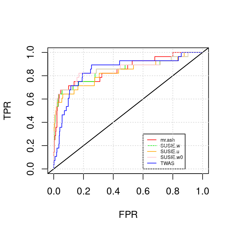

Version	Author	Date
9783727	simingz	2020-08-06
958f794	simingz	2020-08-05
89b90ad	simingz	2020-07-24

AUC for  mr.ash :  0.8532693AUC for  SUSIE.w :  0.8479238AUC for  SUSIE.u :  0.8314224AUC for  SUSIE.w0 :  0.8593121AUC for  TWAS :  0.8474589

NULL; snp-expr; expr-snp

ROC_plot(tags = tags, tag2 = tag2s[2])

Version	Author	Date
9783727	simingz	2020-08-06
958f794	simingz	2020-08-05
89b90ad	simingz	2020-07-24

AUC for  mr.ash :  0.8532693AUC for  SUSIE.w :  0.8479238AUC for  SUSIE.u :  0.8314224AUC for  SUSIE.w0 :  0.8593121AUC for  TWAS :  0.8474589

lasso; expr-snp; expr-snp

ROC_plot(tags = tags, tag2 = tag2s[3])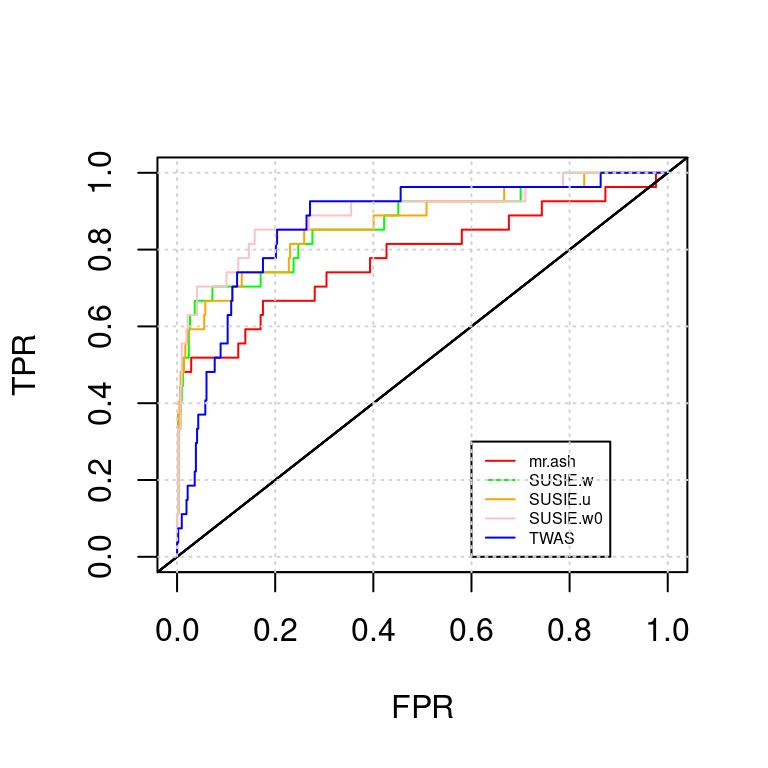

Version	Author	Date
9783727	simingz	2020-08-06
958f794	simingz	2020-08-05
89b90ad	simingz	2020-07-24

AUC for  mr.ash :  0.7802647AUC for  SUSIE.w :  0.8690825AUC for  SUSIE.u :  0.8678391AUC for  SUSIE.w0 :  0.8949285AUC for  TWAS :  0.8674838

lasso; expr-snp; snp-expr

ROC_plot(tags = tags, tag2 = tag2s[4])

Version	Author	Date
9783727	simingz	2020-08-06
958f794	simingz	2020-08-05
89b90ad	simingz	2020-07-24

AUC for  mr.ash :  0.7769784AUC for  SUSIE.w :  0.8691713AUC for  SUSIE.u :  0.8678391AUC for  SUSIE.w0 :  0.8948397AUC for  TWAS :  0.8674838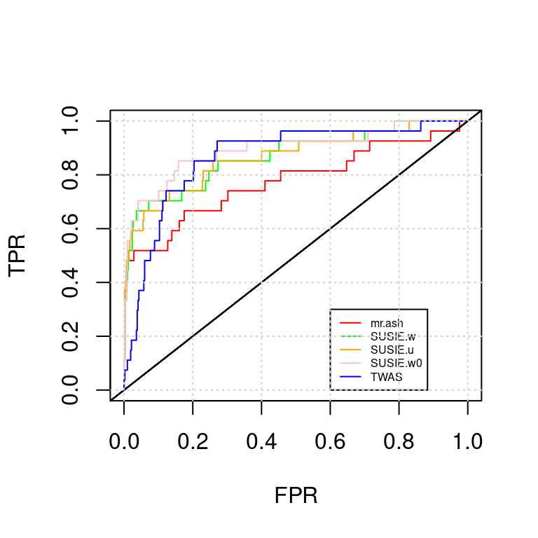

PIP vs p value

NULL; expr-snp; expr-snp

scatter_plot_PIP_p(tags, tag2s[1])

sessionInfo()

R version 3.5.1 (2018-07-02)
Platform: x86_64-pc-linux-gnu (64-bit)
Running under: Scientific Linux 7.4 (Nitrogen)

Matrix products: default
BLAS/LAPACK: /software/openblas-0.2.19-el7-x86_64/lib/libopenblas_haswellp-r0.2.19.so

locale:
 [1] LC_CTYPE=en_US.UTF-8       LC_NUMERIC=C              
 [3] LC_TIME=en_US.UTF-8        LC_COLLATE=en_US.UTF-8    
 [5] LC_MONETARY=en_US.UTF-8    LC_MESSAGES=en_US.UTF-8   
 [7] LC_PAPER=en_US.UTF-8       LC_NAME=C                 
 [9] LC_ADDRESS=C               LC_TELEPHONE=C            
[11] LC_MEASUREMENT=en_US.UTF-8 LC_IDENTIFICATION=C       

attached base packages:
[1] stats     graphics  grDevices utils     datasets  methods   base     

other attached packages:
[1] kableExtra_1.1.0    stringr_1.4.0       plyr_1.8.6         
[4] tidyr_0.8.3         plotly_4.9.2.9000   ggplot2_3.3.1      
[7] data.table_1.12.7   mr.ash.alpha_0.1-34

loaded via a namespace (and not attached):
 [1] tidyselect_1.1.0  purrr_0.3.4       lattice_0.20-38  
 [4] colorspace_1.3-2  vctrs_0.3.1       generics_0.0.2   
 [7] htmltools_0.3.6   viridisLite_0.3.0 yaml_2.2.0       
[10] rlang_0.4.6       later_0.7.5       pillar_1.4.4     
[13] glue_1.4.1        withr_2.1.2       lifecycle_0.2.0  
[16] munsell_0.5.0     gtable_0.2.0      workflowr_1.6.2  
[19] rvest_0.3.2       htmlwidgets_1.3   evaluate_0.12    
[22] knitr_1.20        crosstalk_1.0.0   httpuv_1.4.5     
[25] highr_0.7         Rcpp_1.0.4.6      xtable_1.8-3     
[28] readr_1.3.1       promises_1.0.1    scales_1.0.0     
[31] backports_1.1.2   webshot_0.5.1     jsonlite_1.6.1   
[34] mime_0.6          fs_1.3.1          hms_0.4.2        
[37] digest_0.6.25     stringi_1.3.1     shiny_1.2.0      
[40] dplyr_1.0.0       grid_3.5.1        rprojroot_1.3-2  
[43] tools_3.5.1       magrittr_1.5      lazyeval_0.2.1   
[46] tibble_3.0.1      crayon_1.3.4      whisker_0.3-2    
[49] pkgconfig_2.0.2   ellipsis_0.3.1    Matrix_1.2-15    
[52] xml2_1.2.0        rmarkdown_1.10    httr_1.4.1       
[55] rstudioapi_0.11   R6_2.3.0          git2r_0.26.1     
[58] compiler_3.5.1

Summarize twas: chr22

2020-08-10

Mr.ash2 parameter estimation

NULL; expr-snp; expr-snp

NULL; snp-expr; expr-snp

lasso; expr-snp; expr-snp

lasso; expr-snp; snp-expr

Regional mr.ash2s PIP overview

PIP calibration

NULL; expr-snp; expr-snp

Lasso; expr-snp; expr-snp

PIP scatter plot

NULL; expr-snp; expr-snp

NULL; snp-expr; expr-snp

lasso; expr-snp; expr-snp

lasso; expr-snp; snp-expr

ROC curve

NULL; expr-snp; expr-snp

NULL; snp-expr; expr-snp

lasso; expr-snp; expr-snp

lasso; expr-snp; snp-expr

PIP vs p value

NULL; expr-snp; expr-snp