Summarize twas: chr17 to 22
2020-09-08
Last updated: 2020-09-08
Checks: 6 1
Knit directory: causal-TWAS/
This reproducible R Markdown analysis was created with workflowr (version 1.6.2). The Checks tab describes the reproducibility checks that were applied when the results were created. The Past versions tab lists the development history.
The R Markdown file has unstaged changes. To know which version of the R Markdown file created these results, you’ll want to first commit it to the Git repo. If you’re still working on the analysis, you can ignore this warning. When you’re finished, you can run wflow_publish to commit the R Markdown file and build the HTML.
Great job! The global environment was empty. Objects defined in the global environment can affect the analysis in your R Markdown file in unknown ways. For reproduciblity it’s best to always run the code in an empty environment.
The command set.seed(20191103) was run prior to running the code in the R Markdown file. Setting a seed ensures that any results that rely on randomness, e.g. subsampling or permutations, are reproducible.
Great job! Recording the operating system, R version, and package versions is critical for reproducibility.
Nice! There were no cached chunks for this analysis, so you can be confident that you successfully produced the results during this run.
Great job! Using relative paths to the files within your workflowr project makes it easier to run your code on other machines.
Great! You are using Git for version control. Tracking code development and connecting the code version to the results is critical for reproducibility.
The results in this page were generated with repository version a594e26. See the Past versions tab to see a history of the changes made to the R Markdown and HTML files.
Note that you need to be careful to ensure that all relevant files for the analysis have been committed to Git prior to generating the results (you can use wflow_publish or wflow_git_commit). workflowr only checks the R Markdown file, but you know if there are other scripts or data files that it depends on. Below is the status of the Git repository when the results were generated:
Ignored files:
    Ignored:    .Rhistory
    Ignored:    .Rproj.user/
    Ignored:    code/workflow/.ipynb_checkpoints/
    Ignored:    data/

Unstaged changes:
    Modified:   analysis/description.Rmd
    Modified:   analysis/index.Rmd
    Modified:   analysis/simulation-multi-ukbchr17to22-gtex.adipose_sa2_v2.Rmd
Note that any generated files, e.g. HTML, png, CSS, etc., are not included in this status report because it is ok for generated content to have uncommitted changes.
These are the previous versions of the repository in which changes were made to the R Markdown (analysis/simulation-multi-ukbchr17to22-gtex.adipose_sa2_v2.Rmd) and HTML (docs/simulation-multi-ukbchr17to22-gtex.adipose_sa2_v2.html) files. If you’ve configured a remote Git repository (see ?wflow_git_remote), click on the hyperlinks in the table below to view the files as they were in that past version.
| File | Version | Author | Date | Message |
|---|---|---|---|---|
| Rmd | a594e26 | simingz | 2020-09-06 | pretty plot for Xin’s grant |
| html | a594e26 | simingz | 2020-09-06 | pretty plot for Xin’s grant |
| Rmd | 21378ad | simingz | 2020-09-06 | pretty plot for Xin’s grant |
| html | 21378ad | simingz | 2020-09-06 | pretty plot for Xin’s grant |
| Rmd | fd909a1 | simingz | 2020-08-14 | susieI |
| html | 1d3e1ed | simingz | 2020-08-10 | clean |
| Rmd | 9783727 | simingz | 2020-08-06 | susie names |
| html | 9783727 | simingz | 2020-08-06 | susie names |
| Rmd | 2216650 | simingz | 2020-08-06 | Remove ignored files |
| html | 2216650 | simingz | 2020-08-06 | Remove ignored files |
| Rmd | b6132ab | simingz | 2020-08-05 | visual chr17to22 |
| html | b6132ab | simingz | 2020-08-05 | visual chr17to22 |
| Rmd | 958f794 | simingz | 2020-08-05 | move code- plot functions |
| html | 958f794 | simingz | 2020-08-05 | move code- plot functions |
| Rmd | 86e42c2 | simingz | 2020-08-04 | website hide code |
| html | 86e42c2 | simingz | 2020-08-04 | website hide code |
| Rmd | f6ea15c | simingz | 2020-08-04 | change sa2 grid |
| html | f6ea15c | simingz | 2020-08-04 | change sa2 grid |
`
Run simulation 8 times for ukb chr 17 to chr 22 combined. SNPs are downsampled to 1/10, eQTLs defined by FUSION-TWAS (Adipose/GTEx) lasso effect size > 0 were kept, p= 86k, n = 20k.
library(mr.ash.alpha)
library(data.table)
suppressMessages({library(plotly)})
library(tidyr)
library(plyr)
library(stringr)
library(kableExtra)
source("analysis/summarize_twas_plots.R")
simdatadir <- "~/causalTWAS/simulations/simulation_ashtest_20200721/"
outputdir <- "~/causalTWAS/simulations/simulation_ashtest_20200721/"
susiedir <- "~/causalTWAS/simulations/simulation_susietest_20200721/"
tags <- paste0('20200721-1-', c(2, 4:9))
tagglob <- '20200721-1-*'
tagextr <- '20200721-1-\\d+'
tag2s <- c('zeroes-es', 'zerose-es', 'lassoes-es','lassoes-se')Mr.ash2 parameter estimation
Results for 10 simulations runs, using different initialize and update strategy
NULL; expr-snp; expr-snp
show_param(tags, tag2s[1])| Simulation# | Truth | Est. | Truth | Est. | Truth | Est. | Truth | Est. |
|---|---|---|---|---|---|---|---|---|
| 1 | 0.0502117 | 0.0043097 | 0.0091963 | 0.0003449 | 0.0024981 | 0.0022082 | 0.0437056 | 0.0458391 |
| 2 | 0.0502117 | 0.0433514 | 0.0114605 | 0.0116073 | 0.0024981 | 0.0027771 | 0.0548585 | 0.0342852 |
| 3 | 0.0502117 | 0.0554445 | 0.0110859 | 0.0148455 | 0.0024981 | 0.0016182 | 0.0478479 | 0.0243124 |
| 4 | 0.0502117 | 0.0202643 | 0.0097170 | 0.0111216 | 0.0024981 | 0.0019085 | 0.0580372 | 0.0339128 |
| 5 | 0.0502117 | 0.0373301 | 0.0111216 | 0.0145758 | 0.0024981 | 0.0018831 | 0.0491958 | 0.0309898 |
| 6 | 0.0502117 | 0.0234295 | 0.0110024 | 0.0168935 | 0.0024981 | 0.0029833 | 0.0477211 | 0.0222202 |
| 7 | 0.0502117 | 0.0272243 | 0.0114627 | 0.0127966 | 0.0024981 | 0.0018503 | 0.0513712 | 0.0297764 |
NULL; snp-expr; expr-snp
show_param(tags, tag2s[2])| Simulation# | Truth | Est. | Truth | Est. | Truth | Est. | Truth | Est. |
|---|---|---|---|---|---|---|---|---|
| 1 | 0.0502117 | 0.0043097 | 0.0091963 | 0.0003449 | 0.0024981 | 0.0022082 | 0.0437056 | 0.0458392 |
| 2 | 0.0502117 | 0.0424709 | 0.0114605 | 0.0118770 | 0.0024981 | 0.0025278 | 0.0548585 | 0.0343060 |
| 3 | 0.0502117 | 0.0558006 | 0.0110859 | 0.0146272 | 0.0024981 | 0.0016143 | 0.0478479 | 0.0242827 |
| 4 | 0.0502117 | 0.0202638 | 0.0097170 | 0.0111219 | 0.0024981 | 0.0019085 | 0.0580372 | 0.0339131 |
| 5 | 0.0502117 | 0.0373297 | 0.0111216 | 0.0145756 | 0.0024981 | 0.0018832 | 0.0491958 | 0.0309887 |
| 6 | 0.0502117 | 0.0234320 | 0.0110024 | 0.0168926 | 0.0024981 | 0.0029832 | 0.0477211 | 0.0222190 |
| 7 | 0.0502117 | 0.0068140 | 0.0114627 | 0.0136486 | 0.0024981 | 0.0003761 | 0.0513712 | 0.0377470 |
lasso; expr-snp; expr-snp
show_param(tags, tag2s[3])| Simulation# | Truth | Est. | Truth | Est. | Truth | Est. | Truth | Est. |
|---|---|---|---|---|---|---|---|---|
| 1 | 0.0502117 | 0.0023143 | 0.0091963 | 0.0001921 | 0.0024981 | 0.0019384 | 0.0437056 | 0.0363801 |
| 2 | 0.0502117 | 0.0159417 | 0.0114605 | 0.0012828 | 0.0024981 | 0.0025405 | 0.0548585 | 0.0483650 |
| 3 | 0.0502117 | 0.0588623 | 0.0110859 | 0.0128581 | 0.0024981 | 0.0015320 | 0.0478479 | 0.0239580 |
| 4 | 0.0502117 | 0.0204854 | 0.0097170 | 0.0109340 | 0.0024981 | 0.0018279 | 0.0580372 | 0.0330261 |
| 5 | 0.0502117 | 0.0397177 | 0.0111216 | 0.0148919 | 0.0024981 | 0.0017947 | 0.0491958 | 0.0375966 |
| 6 | 0.0502117 | 0.0283886 | 0.0110024 | 0.0136540 | 0.0024981 | 0.0023833 | 0.0477211 | 0.0276939 |
| 7 | 0.0502117 | 0.0237217 | 0.0114627 | 0.0136598 | 0.0024981 | 0.0018473 | 0.0513712 | 0.0300877 |
lasso; expr-snp; snp-expr
show_param(tags, tag2s[4])| Simulation# | Truth | Est. | Truth | Est. | Truth | Est. | Truth | Est. |
|---|---|---|---|---|---|---|---|---|
| 1 | 0.0502117 | 0.0148369 | 0.0091963 | 0.0061704 | 0.0024981 | 0.0015261 | 0.0437056 | 0.0302851 |
| 2 | 0.0502117 | 0.0383624 | 0.0114605 | 0.0115444 | 0.0024981 | 0.0018645 | 0.0548585 | 0.0391774 |
| 3 | 0.0502117 | 0.0478061 | 0.0110859 | 0.0156099 | 0.0024981 | 0.0011384 | 0.0478479 | 0.0235886 |
| 4 | 0.0502117 | 0.0225364 | 0.0097170 | 0.0127132 | 0.0024981 | 0.0014313 | 0.0580372 | 0.0308298 |
| 5 | 0.0502117 | 0.0392400 | 0.0111216 | 0.0153121 | 0.0024981 | 0.0015686 | 0.0491958 | 0.0371479 |
| 6 | 0.0502117 | 0.0272458 | 0.0110024 | 0.0142985 | 0.0024981 | 0.0019134 | 0.0477211 | 0.0273657 |
| 7 | 0.0502117 | 0.0061805 | 0.0114627 | 0.0124158 | 0.0024981 | 0.0003996 | 0.0513712 | 0.0400624 |
Regional mr.ash2s PIP overview
Take simulation 1 (NULL; expr-snp; expr-snp) as examples. We use region size 500kb and PIP cut off at 0.5 for SUSIE.
chrom = 18
f <- get_files(tag= "20200721-1-3" , tag2 = tag2s[1])
allchr <- read.table(f[["rpip"]], header = T)
a <- allchr[allchr["chrom"]==chrom,]
print(paste("plot for chr", chrom))
[1] "plot for chr 18"par(mar=c(5, 4, 4, 6) + 0.1)
with(a, plot(p0, rPIP, col ='salmon', xlab = "position", ylab= "Sum of PIP", type = 'h', lwd = 2))
par(new = T)
with(a, plot(p0, nCausal, pch =19, col = "darkgreen",axes = FALSE, bty = "n", xlab = "", ylab = ""))
axis(side = 4)
mtext(side = 4, line = 3, 'No. causal signals')
legend("topleft",
legend=c("Mr.ASH PIP", "# Causal"),
lty=c(1,0), pch=c(NA, 19), col=c("salmon", "darkgreen"))
grid()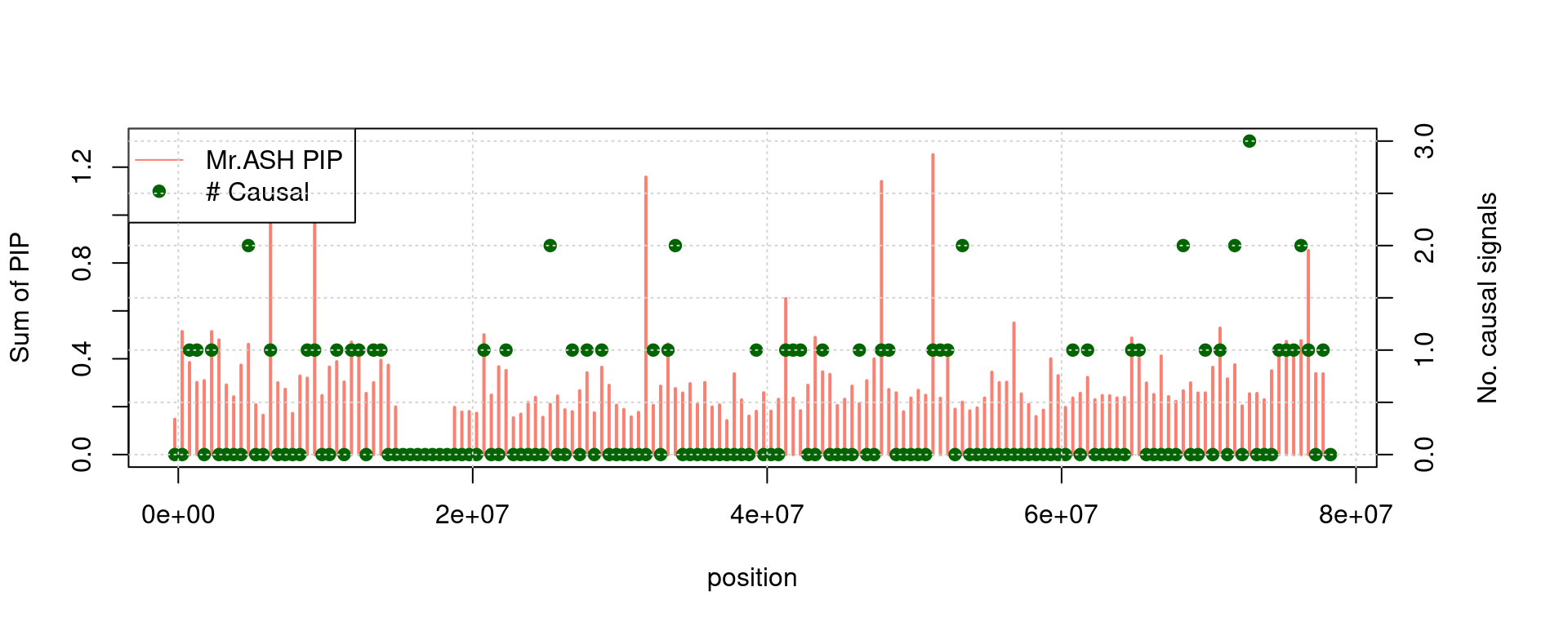
PIP calibration
We run 50 simulations and combine results.
NULL; expr-snp; expr-snp
tag2 = "zeroes-es"
tags_ext <- Reduce(intersect, get_tags(tagglob, tagextr, tag2 = tag2)['gsusie'])
a <- caliPIP_plot(tags = tags_ext, tag2 = tag2)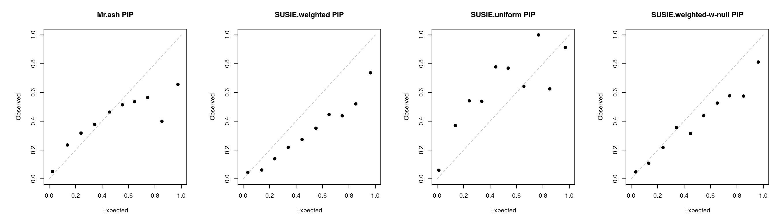
a <- caliFDR_plot(tags = tags_ext, tag2 = tag2)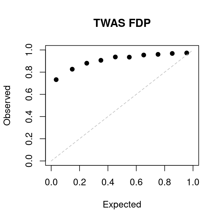
FDR at bonferroni corrected p = 0.05: 0.645933Lasso; expr-snp; expr-snp
a <- caliPIP_plot(tags = tags_ext, tag2 = "lassoes-es")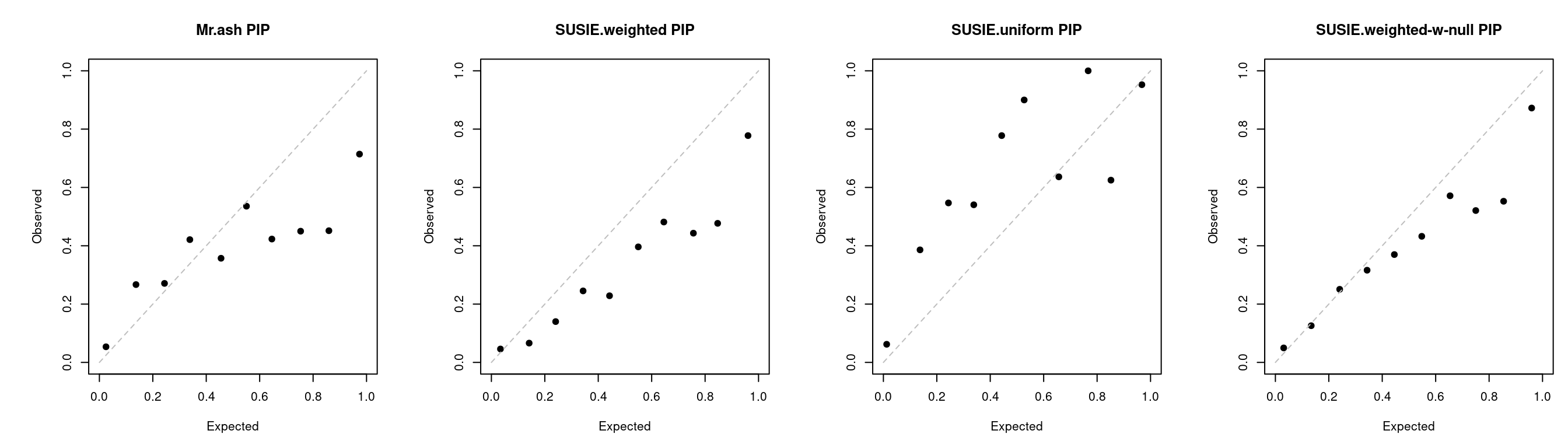
a <- caliFDR_plot(tags = tags_ext, tag2 = "lassoes-es")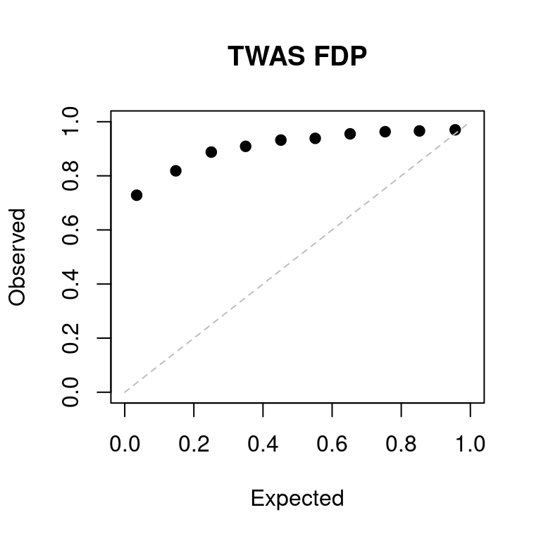
FDR at bonferroni corrected p = 0.05: 0.647343PIP scatter plot
mr.ash2s PIP vs. susie PIP.
NULL; expr-snp; expr-snp
scatter_plot_PIP(tags, tag2s[1])scatter_plot_PIP(tags, tag2s[2])scatter_plot_PIP(tags, tag2s[3])lasso; expr-snp; snp-expr
scatter_plot_PIP(tags, tag2s[4])ROC curve
NULL; expr-snp; expr-snp
tags <- paste0('20200721-1-', c(2,4:9))
ROC_plot(tags, tag2s[2])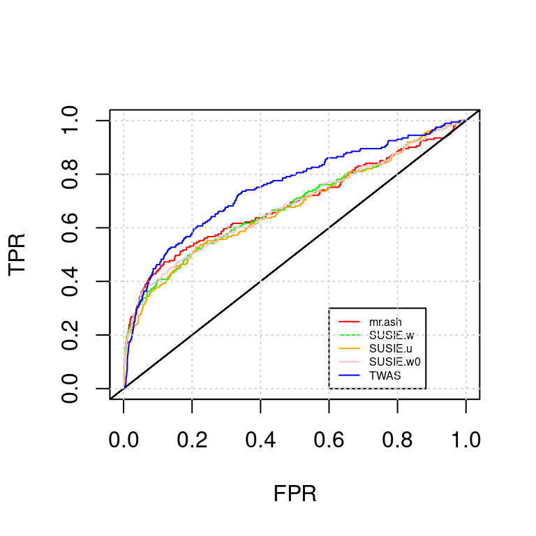
AUC for mr.ash : 0.6894131AUC for SUSIE.w : 0.6824739AUC for SUSIE.u : 0.6762515AUC for SUSIE.w0 : 0.6835701AUC for TWAS : 0.7488581NULL; snp-expr; expr-snp
ROC_plot(tags, tag2s[2])
AUC for mr.ash : 0.6894131AUC for SUSIE.w : 0.6824739AUC for SUSIE.u : 0.6762515AUC for SUSIE.w0 : 0.6835701AUC for TWAS : 0.7488581lasso; expr-snp; expr-snp
ROC_plot(tags, tag2s[3])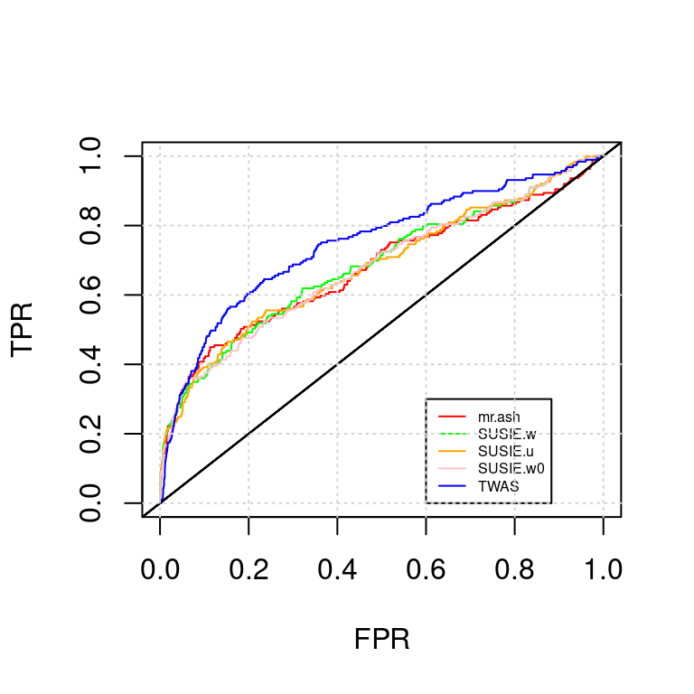
AUC for mr.ash : 0.6778905AUC for SUSIE.w : 0.6857911AUC for SUSIE.u : 0.6818999AUC for SUSIE.w0 : 0.6799617AUC for TWAS : 0.7489982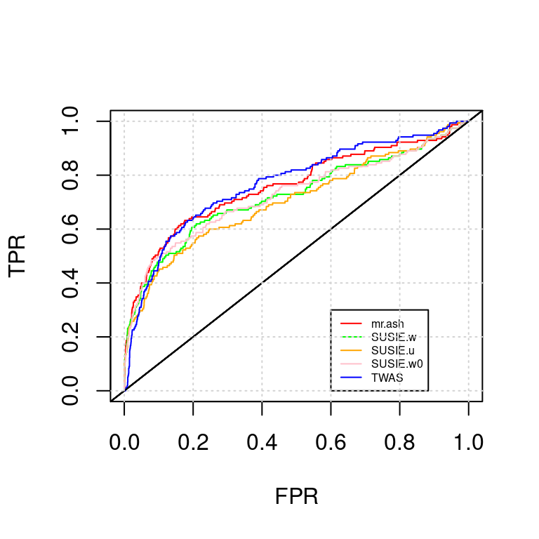
PIP vs p value
Lasso; expr-snp; expr-snp
a <- scatter_plot_PIP_p(tags, "lassoes-es")Pretty plots
- PIP calibration plot; B) FDP inflation of TWAS; C) Scatter plot of individual genes: PIPs vs. -log10-p values from TWAS.
We use SNP genotype data from chr 17 to chr 22 combined. These genomic regions represents 12.5% of the genome. SNPs are downsampled to 1/10 (randomly), eQTLs used in building the expression model were added back. We used lasso to train expression model using GTEx adipose tissue v7. In this simulation, we simulate phenotype with PVE explained by gene as 0.01, by SNP 0.05. pi1 for gene 0.05, pi1 for SNP 0.0025.
For our method, we run mr.ash2s for both genes and SNPs (initiated with lasso). Then apply SUSIE for regions with sum of PIP > 0.5. This gives us PIP for individual genes.
For TWAS, we use linear regression for each gene and obtain p values.
par(mfrow=c(1,3))
cp_plot(res1$SUSIE.w0_PIP, res1$ifcausal, main = "SUSIE PIP calibration", col = "firebrick",cex.lab=1.4, cex.axis=1.4, cex.main=1.4, cex.sub=1.4)
grid()
cp_plot(res2$FDR, res2$ifcausal, mode ="FDR", main = "TWAS FDP", col= "darkgreen",cex.lab=1.4, cex.axis=1.4, cex.main=1.4, cex.sub=1.4)
grid()
plot(res3$TWAS, res3$SUSIE.w0, col = ifelse(res3$ifcausal=="Causal",  "salmon", "cyan3"), xlab = expression('TWAS -log'[10]*'(p)'), ylab = "SUSIE PIP",pch =19,cex.lab=1.4, cex.axis=1.4, cex.main=1.4, cex.sub=1.4)
grid()
legend(8.5, 0.6,
       legend = c("Causal", "Non causal"),
      cex=1.1, pch=19, col=c("salmon", "cyan3"))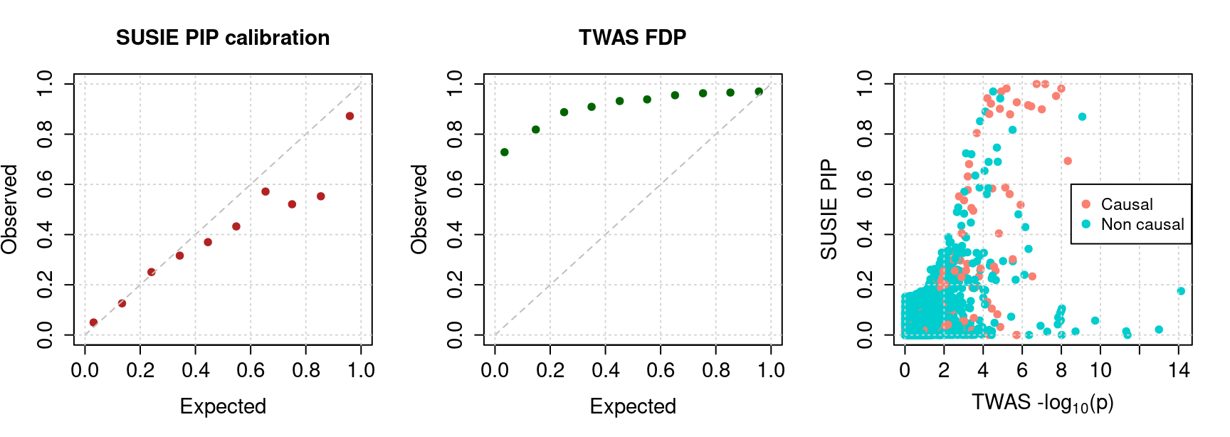
| Version | Author | Date |
|---|---|---|
| 21378ad | simingz | 2020-09-06 |
sessionInfo()R version 3.5.1 (2018-07-02)
Platform: x86_64-pc-linux-gnu (64-bit)
Running under: Scientific Linux 7.4 (Nitrogen)
Matrix products: default
BLAS/LAPACK: /software/openblas-0.2.19-el7-x86_64/lib/libopenblas_haswellp-r0.2.19.so
locale:
[1] LC_CTYPE=en_US.UTF-8 LC_NUMERIC=C
[3] LC_TIME=en_US.UTF-8 LC_COLLATE=en_US.UTF-8
[5] LC_MONETARY=en_US.UTF-8 LC_MESSAGES=en_US.UTF-8
[7] LC_PAPER=en_US.UTF-8 LC_NAME=C
[9] LC_ADDRESS=C LC_TELEPHONE=C
[11] LC_MEASUREMENT=en_US.UTF-8 LC_IDENTIFICATION=C
attached base packages:
[1] stats graphics grDevices utils datasets methods base
other attached packages:
[1] kableExtra_1.2.1 stringr_1.4.0 plyr_1.8.6
[4] tidyr_0.8.3 plotly_4.9.2.9000 ggplot2_3.3.1
[7] data.table_1.12.7 mr.ash.alpha_0.1-34
loaded via a namespace (and not attached):
[1] tidyselect_1.1.0 purrr_0.3.4 lattice_0.20-38
[4] colorspace_1.3-2 vctrs_0.3.1 generics_0.0.2
[7] htmltools_0.3.6 viridisLite_0.3.0 yaml_2.2.0
[10] rlang_0.4.6 later_0.7.5 pillar_1.4.4
[13] glue_1.4.1 withr_2.1.2 lifecycle_0.2.0
[16] munsell_0.5.0 gtable_0.2.0 workflowr_1.6.2
[19] rvest_0.3.2 htmlwidgets_1.3 evaluate_0.12
[22] knitr_1.20 crosstalk_1.0.0 httpuv_1.4.5
[25] highr_0.7 Rcpp_1.0.4.6 xtable_1.8-3
[28] promises_1.0.1 scales_1.0.0 backports_1.1.2
[31] webshot_0.5.1 jsonlite_1.6.1 mime_0.6
[34] fs_1.3.1 digest_0.6.25 stringi_1.3.1
[37] shiny_1.2.0 dplyr_1.0.0 grid_3.5.1
[40] rprojroot_1.3-2 tools_3.5.1 magrittr_1.5
[43] lazyeval_0.2.1 tibble_3.0.1 crayon_1.3.4
[46] whisker_0.3-2 pkgconfig_2.0.2 ellipsis_0.3.1
[49] Matrix_1.2-15 xml2_1.2.0 rmarkdown_1.10
[52] httr_1.4.1 rstudioapi_0.11 R6_2.3.0
[55] git2r_0.26.1 compiler_3.5.1