Simulations to test ctwas summary stats version, 45k samples
Last updated: 2021-08-04
Checks: 5 2
Knit directory: causal-TWAS/
This reproducible R Markdown analysis was created with workflowr (version 1.6.2). The Checks tab describes the reproducibility checks that were applied when the results were created. The Past versions tab lists the development history.
The R Markdown file has unstaged changes. To know which version of the R Markdown file created these results, you'll want to first commit it to the Git repo. If you're still working on the analysis, you can ignore this warning. When you're finished, you can run wflow_publish to commit the R Markdown file and build the HTML.
Great job! The global environment was empty. Objects defined in the global environment can affect the analysis in your R Markdown file in unknown ways. For reproduciblity it's best to always run the code in an empty environment.
The command set.seed(20191103) was run prior to running the code in the R Markdown file. Setting a seed ensures that any results that rely on randomness, e.g. subsampling or permutations, are reproducible.
Great job! Recording the operating system, R version, and package versions is critical for reproducibility.
Nice! There were no cached chunks for this analysis, so you can be confident that you successfully produced the results during this run.
Using absolute paths to the files within your workflowr project makes it difficult for you and others to run your code on a different machine. Change the absolute path(s) below to the suggested relative path(s) to make your code more reproducible.
| absolute | relative |
|---|---|
| ~/causalTWAS/causal-TWAS/analysis/summarize_ctwas_plots.R | analysis/summarize_ctwas_plots.R |
| ~/causalTWAS/causal-TWAS/analysis/summarize_twas-coloc_plots.R | analysis/summarize_twas-coloc_plots.R |
| ~/causalTWAS/causal-TWAS/analysis/summarize_focus_plots.R | analysis/summarize_focus_plots.R |
| ~/causalTWAS/causal-TWAS/analysis/summarize_smr_plots.R | analysis/summarize_smr_plots.R |
| ~/causalTWAS/causal-TWAS/analysis/summarize_mrjti_plots.R | analysis/summarize_mrjti_plots.R |
| ~/causalTWAS/causal-TWAS/code/qqplot.R | code/qqplot.R |
Great! You are using Git for version control. Tracking code development and connecting the code version to the results is critical for reproducibility.
The results in this page were generated with repository version 8521449. See the Past versions tab to see a history of the changes made to the R Markdown and HTML files.
Note that you need to be careful to ensure that all relevant files for the analysis have been committed to Git prior to generating the results (you can use wflow_publish or wflow_git_commit). workflowr only checks the R Markdown file, but you know if there are other scripts or data files that it depends on. Below is the status of the Git repository when the results were generated:
Ignored files:
    Ignored:    .Rhistory
    Ignored:    .Rproj.user/
    Ignored:    .ipynb_checkpoints/
    Ignored:    analysis/.ipynb_checkpoints/
    Ignored:    code/.ipynb_checkpoints/
    Ignored:    code/before_package/.ipynb_checkpoints/
    Ignored:    code/workflow/.ipynb_checkpoints/
    Ignored:    data/

Unstaged changes:
    Modified:   analysis/simulation-ctwas-ukbWG-gtex.adipose_s80.45_041621.Rmd
Note that any generated files, e.g. HTML, png, CSS, etc., are not included in this status report because it is ok for generated content to have uncommitted changes.
These are the previous versions of the repository in which changes were made to the R Markdown (analysis/simulation-ctwas-ukbWG-gtex.adipose_s80.45_041621.Rmd) and HTML (docs/simulation-ctwas-ukbWG-gtex.adipose_s80.45_041621.html) files. If you've configured a remote Git repository (see ?wflow_git_remote), click on the hyperlinks in the table below to view the files as they were in that past version.
| File | Version | Author | Date | Message |
|---|---|---|---|---|
| Rmd | 6dee9b0 | simingz | 2021-07-22 | bonferroni Fusion, description |
| html | 6dee9b0 | simingz | 2021-07-22 | bonferroni Fusion, description |
| Rmd | 18f165e | simingz | 2021-06-15 | LDR2.R |
| Rmd | b948950 | simingz | 2021-06-07 | matching ctwas v0.1.29 |
| Rmd | fe0e8f8 | simingz | 2021-05-09 | added smr-heidi results, scripts matching v0.1.25 |
| html | fe0e8f8 | simingz | 2021-05-09 | added smr-heidi results, scripts matching v0.1.25 |
| Rmd | f9eedf9 | simingz | 2021-04-21 | focus results |
library(ctwas)
library(data.table)
suppressMessages({library(plotly)})
library(tidyr)
library(plyr)
library(stringr)
source("~/causalTWAS/causal-TWAS/analysis/summarize_ctwas_plots.R")
source('~/causalTWAS/causal-TWAS/analysis/summarize_twas-coloc_plots.R')
source('~/causalTWAS/causal-TWAS/analysis/summarize_focus_plots.R')
source('~/causalTWAS/causal-TWAS/analysis/summarize_smr_plots.R')
source('~/causalTWAS/causal-TWAS/analysis/summarize_mrjti_plots.R')
source('~/causalTWAS/causal-TWAS/code/qqplot.R')
pgenfn = "/home/simingz/causalTWAS/ukbiobank/ukb_pgen_s80.45/ukb-s80.45_pgenfs.txt"
ld_pgenfn = "/home/simingz/causalTWAS/ukbiobank/ukb_pgen_s80.45/ukb-s80.45.2_pgenfs.txt"
outputdir = "/home/simingz/causalTWAS/simulations/simulation_ctwas_rss_20210416/" # /
comparedir = "/home/simingz/causalTWAS/simulations/simulation_ctwas_rss_20210416_compare/"
runtag = "ukb-s80.45-adi"
configtags = 1
simutags = paste(rep(1:2, each = length(1:5)), 1:5, sep = "-")
pgenfs <- read.table(pgenfn, header = F, stringsAsFactors = F)[,1]
pvarfs <- sapply(pgenfs, prep_pvar, outputdir = outputdir)
ld_pgenfs <- read.table(ld_pgenfn, header = F, stringsAsFactors = F)[,1]
ld_pvarfs <- sapply(ld_pgenfs, prep_pvar, outputdir = outputdir)
pgens <- lapply(1:length(pgenfs), function(x) prep_pgen(pgenf = pgenfs[x],pvarf = pvarfs[x]))Analysis description
n.ori <- 80000 # number of samples
n <- pgenlibr::GetRawSampleCt(pgens[[1]])
p <- sum(unlist(lapply(pgens, pgenlibr::GetVariantCt))) # number of SNPs
J <- 8021 # number of genes
Data
- GWAS summary statistics we simulated summary statistics data with different causal gene/SNP proportion and PVE. To simulate this data, we need the following:
- genotype data we used is from UKB biobank, randomly selecting 80000 samples. We then filtered samples. The columns selected for filtering samples are as follows:
- sex (31)
- UK Biobank assessment centre (54)
- age (21022)
- genetic ethnic grouping (22006)
- genetic sex (22001)
- genotype measurement batch (22000)
- missingness (22005)
- genetic PCs (22009-0.1 - 22009-0.40)
- genetic relatedness pairing (22011)
- genetic kinship (22021)
- outliers (22027)
- Remove all rows in which one or more of the values are missing, aside from the in the "outlier" and "relatedness_genetic" columns. This step removes any samples that are not marked as being "White British".
- Remove rows with mismatches between self-reported and genetic sex
- Remove "missingness" and "heterozygosity" outliers as defined by UK Biobank.
- Remove any individuals have at least one relative
- Remove any individuals that have close relatives identified from the "relatendess" calculations that weren't already identified using the kinship calculations.
- Expression models The one we used in this analysis is GTEx Adipose tissue v7 dataset. This dataset contains ~ 380 samples, 8021 genes with expression model. FUSION/TWAS were used to train expression model and we used their lasso results. SNPs included in eQTL anlaysis are restricted to cis-locus 500kb on either side of the gene boundary. eQTLs are defined as SNPs with abs(effectize) > 1e-8 in lasso results.
To simulate phenotype data, first we impute gene expression based on expression models, then we set gene/SNP pi1 and PVE, get rough effect size for causal SNPs and genes and simulate phenotype under the sparse model with spike and slab prior. Then we performed GWAS for all SNPs and get z scores for each by univariate linear regression.
- genotype data we used is from UKB biobank, randomly selecting 80000 samples. We then filtered samples. The columns selected for filtering samples are as follows:
LD genotype reference We used the genotype of 2k samples from UKbiobank (randomly selected from the samples used in simulations) to serve as the LD reference.
Expression models
We used GTEx Adipose tissue v7 dataset, the same as used for simulating phenotypes.
Analysis
ctwas
Get z scores for gene expression. We used expression models and LD reference to get z scores for gene expression.
Run ctwas_rss
ctwas_rssalgorithm first runs on all regions to get rough estimate for gene and SNP prior. Then run on small regions (having small probablities of having > 1 causal signals based on rough estimates) to get more accurate estimate. To lower computational burden, we downsampled SNPs (0.1) to estimate parameters. With the estimated parameters, we then run susie for all regions using both genes and downsampled SNPs with specified \(L\). After this, for regions with strong gene signals, we rerun susie with full SNPs using specified \(L\).
Configurations
ld_regions ='EUR', We used LDetect to define regions. To match UKbiobank data, we use the 'EUR' population
thin = 0.1, downsampled SNPs to 1/10 for parameter estimation step
niter1 =3, run niter1 =3 iterations first to get some rough parameter estimates.
prob_single = 0.8, the probability of a region having at most 1 singal has to be at least 0.8 to be selected for the parameter estimation step. This probability is obtained by using the PIPs from the first few iterations.
niter2 = 30, run niter2 = 30 for parameter estimation step
L = 3 , after parameter estimation, for running susie for all regions.
group_prior = NULL, the intiating prior parameters we used for running susie for each region is uniform prior for genes and SNPs.
group_prior_var = NULL, the intiating prior variance parameters we used for running susie for each region follows susie_rss's default (50).
max_SNP_region = 5000, the maximum number of SNPs for re-running susie on strong gene signal regions is 5000.
Power estimation
simutag <- "1-1"
niter <- 1000
snp.p <- 5e-8
gene.p <- 1e-5
source(paste0(outputdir, "simu", simutag, "_param.R"))
load(paste0(outputdir, runtag, "_simu", simutag, "-pheno.Rd"))
We select run 1-1 as an example.
- For SNPs. \(\pi_1 =\) 2.510^{-4} , effect size = 0.0283342, PVE = 0.4875046. Power at 5e-08 p value cutoff:
load("data/power_s80.45.Rd")
# p1 <- pow(niter, n, phenores[["batch"]][[1]][["sigma_theta"]], snp.p)
print(p1)
[1] 0.159- For genes. \(\pi_1 = 0.05\) , effect size = 0.0248146, PVE = 0.0922345. Power at 1e-05 p value cutoff:
# p2 <- pow(niter, n, phenores[["batch"]][[1]][["sigma_beta"]], gene.p)
print(p2)
[1] 0.2# save(p1,p2, file = "data/power_s80.45.Rd")GWAS/TWAS p value distribution
simutag <- "1-1"
chrom <- 1
source(paste0(outputdir, "simu", simutag, "_param.R"))
load(paste0(outputdir, runtag, "_simu", simutag, "-pheno.Rd"))
We select run 1-1 as an example.
- For genes. \(\pi_1 = 0.05\) , effect size = 0.0248146, PVE = 0.0922345. TWAS p values and qqplot:
exprgwasf <- paste0(outputdir, runtag, "_simu", simutag, ".exprgwas.txt.gz")

exprvarf <- paste0(outputdir, runtag, "_chr", chrom, ".exprvar")
exprid <- read_exprvar(exprvarf)[, "id"]
cau <- as.matrix(exprid[phenores[["batch"]][[chrom]][["idx.cgene"]]])
pdist_plot(exprgwasf, chrom, cau)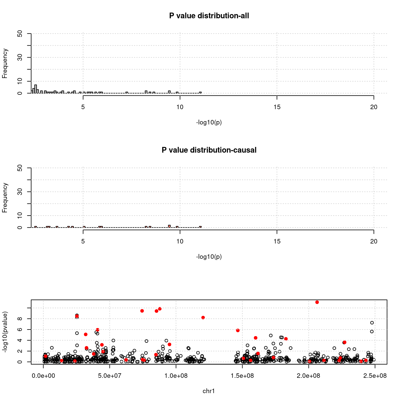
exprgwas <- fread(exprgwasf, header =T)
gg_qqplot(exprgwas$PVALUE)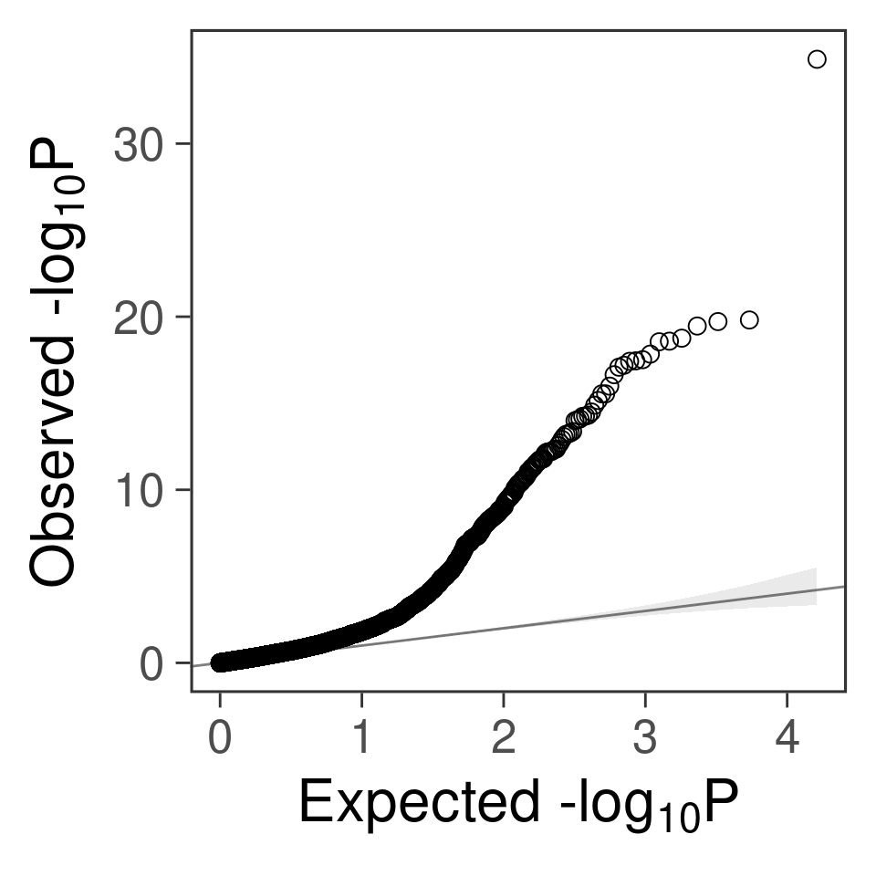
- For SNPs. \(\pi_1 =\) 2.510^{-4} , effect size = 0.0283342, PVE = 0.4875046. GWAS p values and qqplot:
snpgwasf <-  paste0(outputdir, runtag, "_simu", simutag, ".snpgwas.txt.gz")

pvarf <- pvarfs[chrom]
snpid <- read_pvar(pvarf)[, "id"]
cau <- as.matrix(snpid[phenores[["batch"]][[chrom]][["idx.cSNP"]]])
pdist_plot(snpgwasf, chrom, cau, thin = 0.1)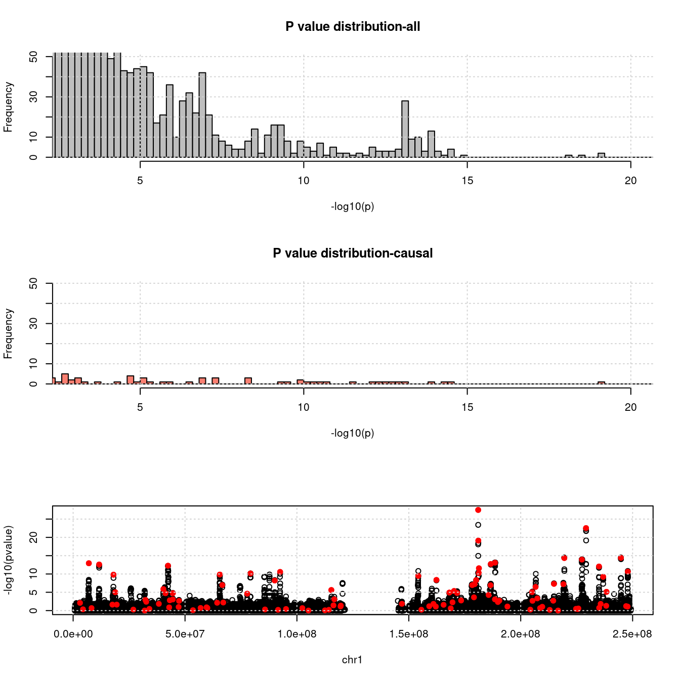
snpgwas <- fread(snpgwasf, header =T)
gg_qqplot(snpgwas$PVALUE, thin = 0.1)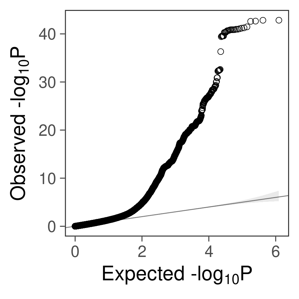
ctwas results
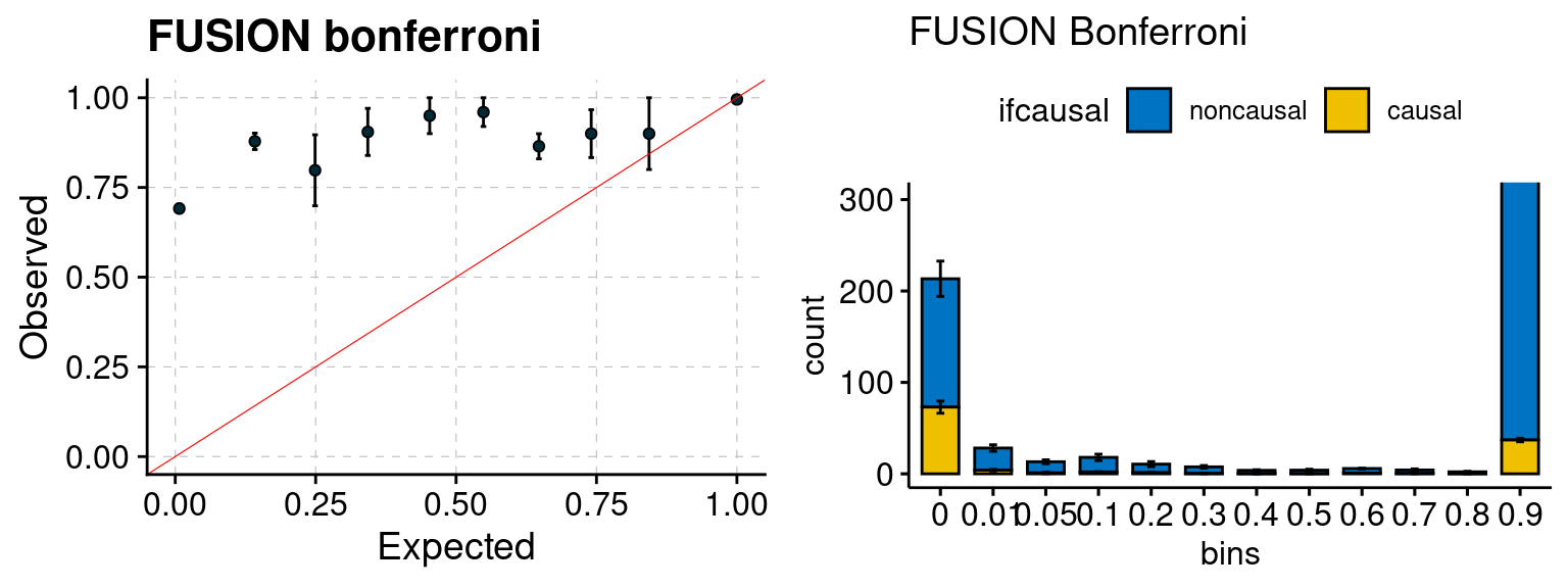
Results: Each row shows parameter estimation results from 5 simulation runs with similar settings (i.e. pi1 and PVE for genes and SNPs). Results from each run were represented by one dot, dots with the same color come from the same run. truth: the true parameters, selected_truth: the truth in selected regions that were used to estimate parameters, ctwas: ctwas estimated parameters (using summary statistics as input). We run FUSION following default settings and adjust p values by BH method to get expected FDP.
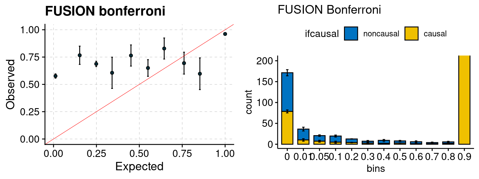
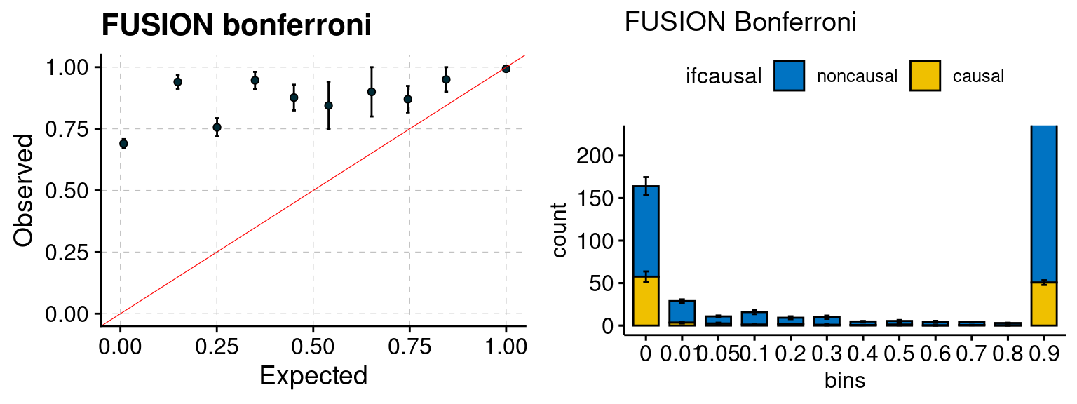
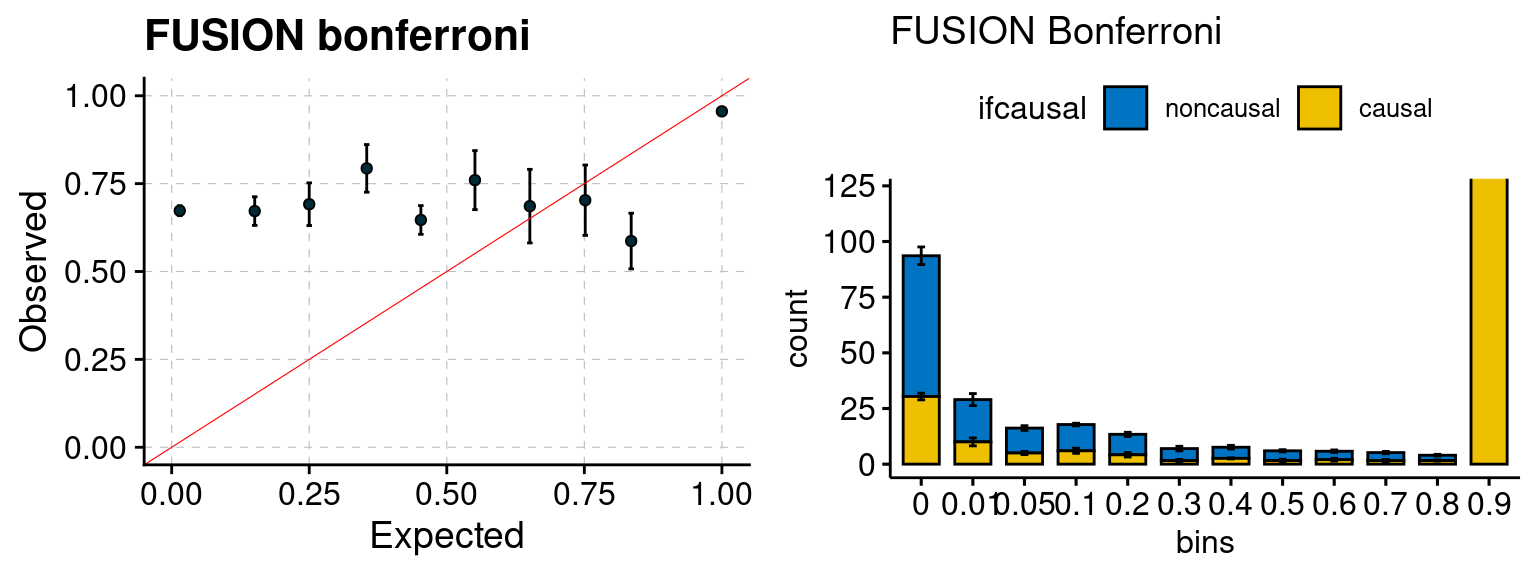
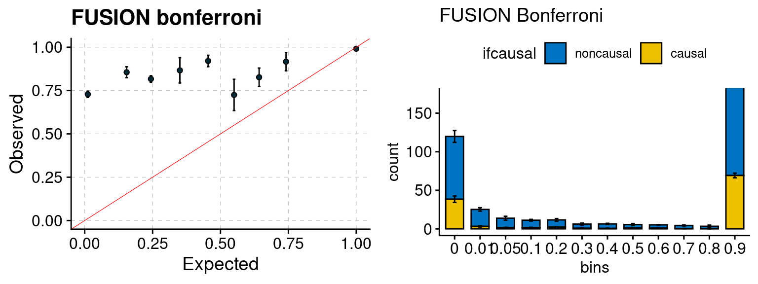
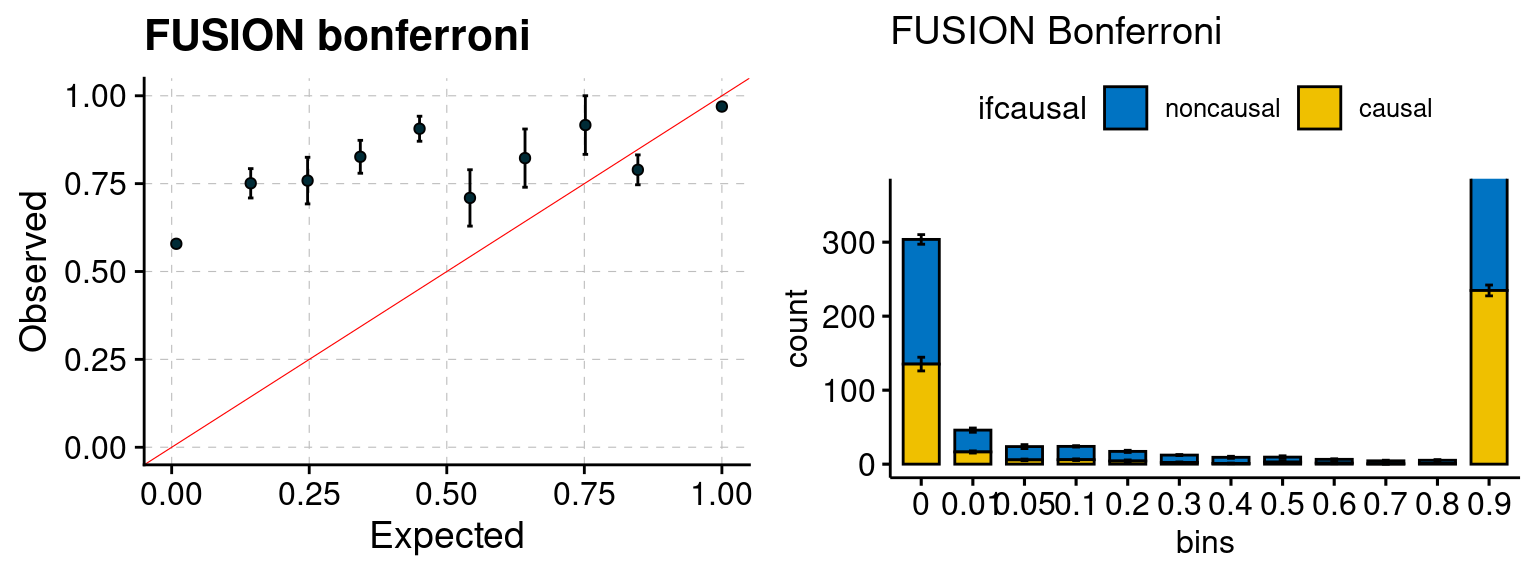
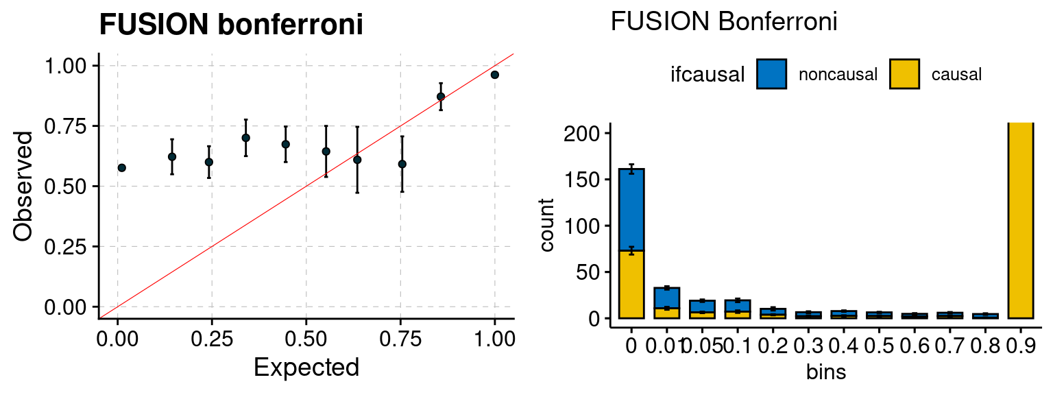
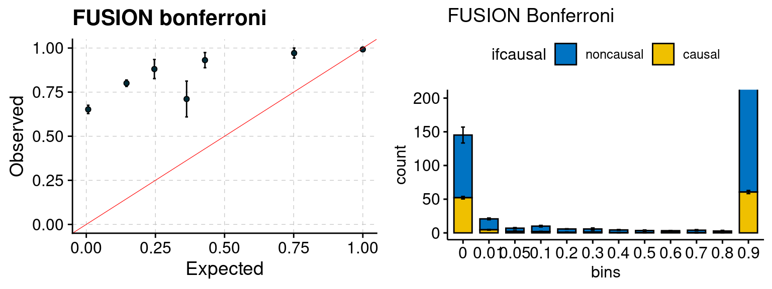
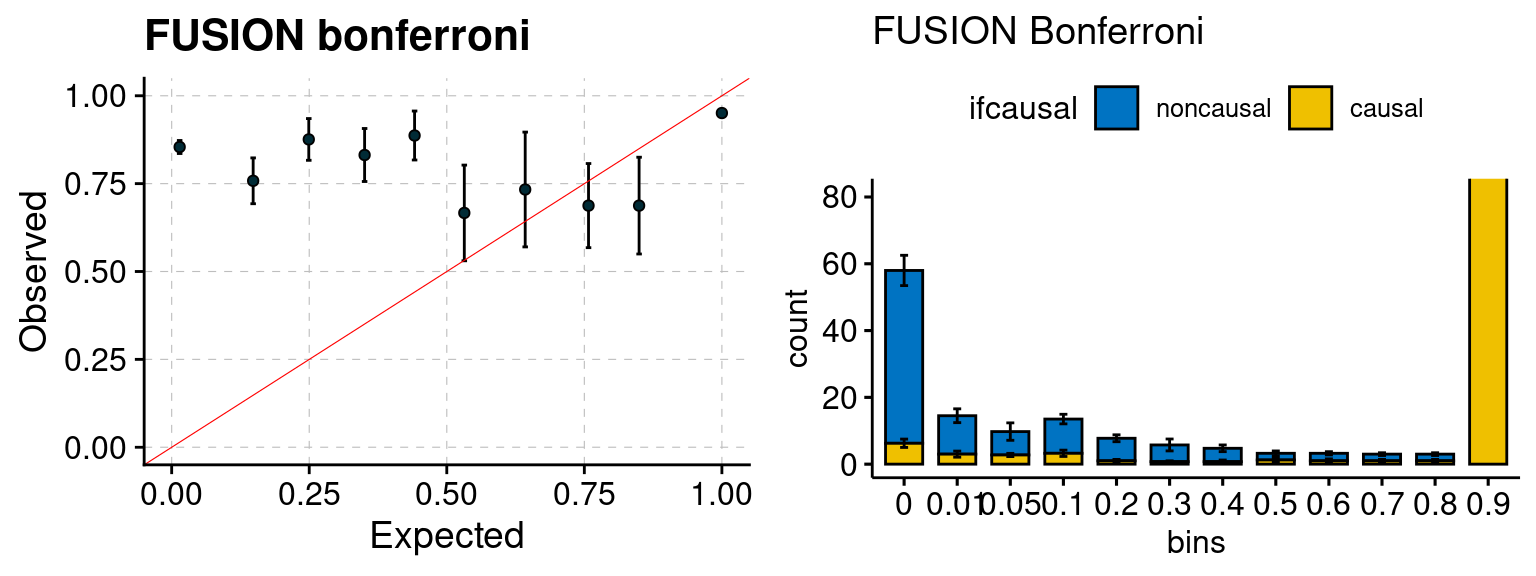
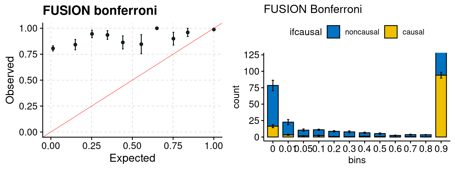
We run FUSION following default settings and adjust p values by BH method to get expected FDP. We have also used Bonferroni correction for p values.
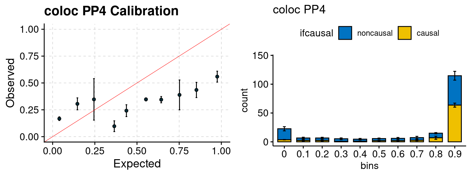
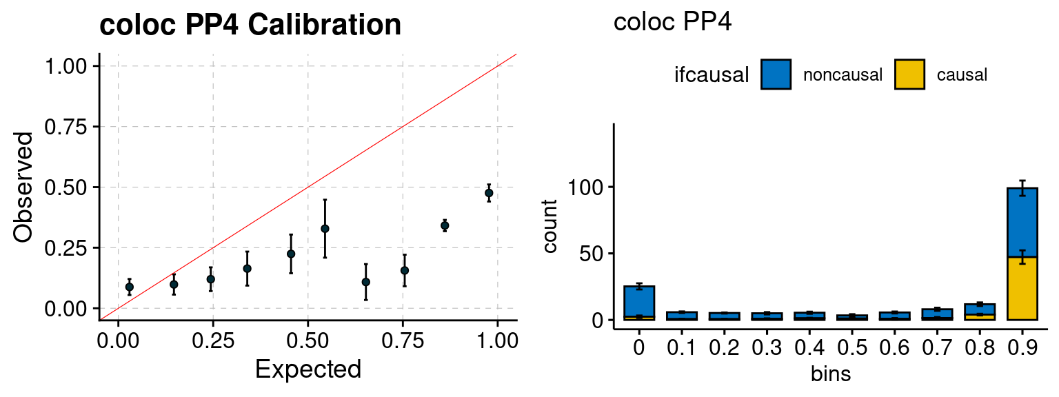
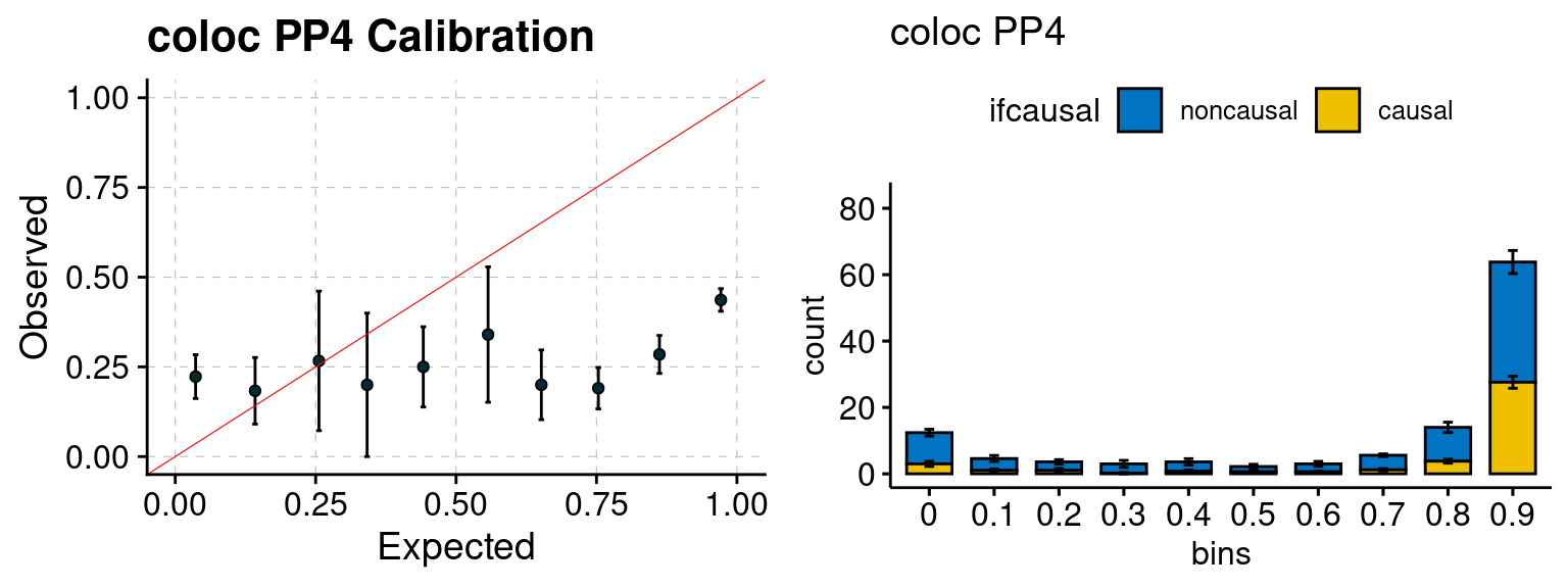
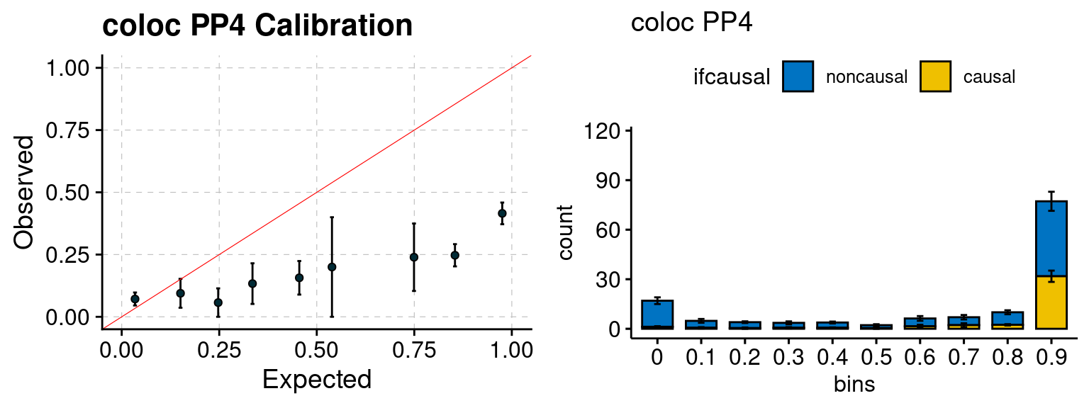
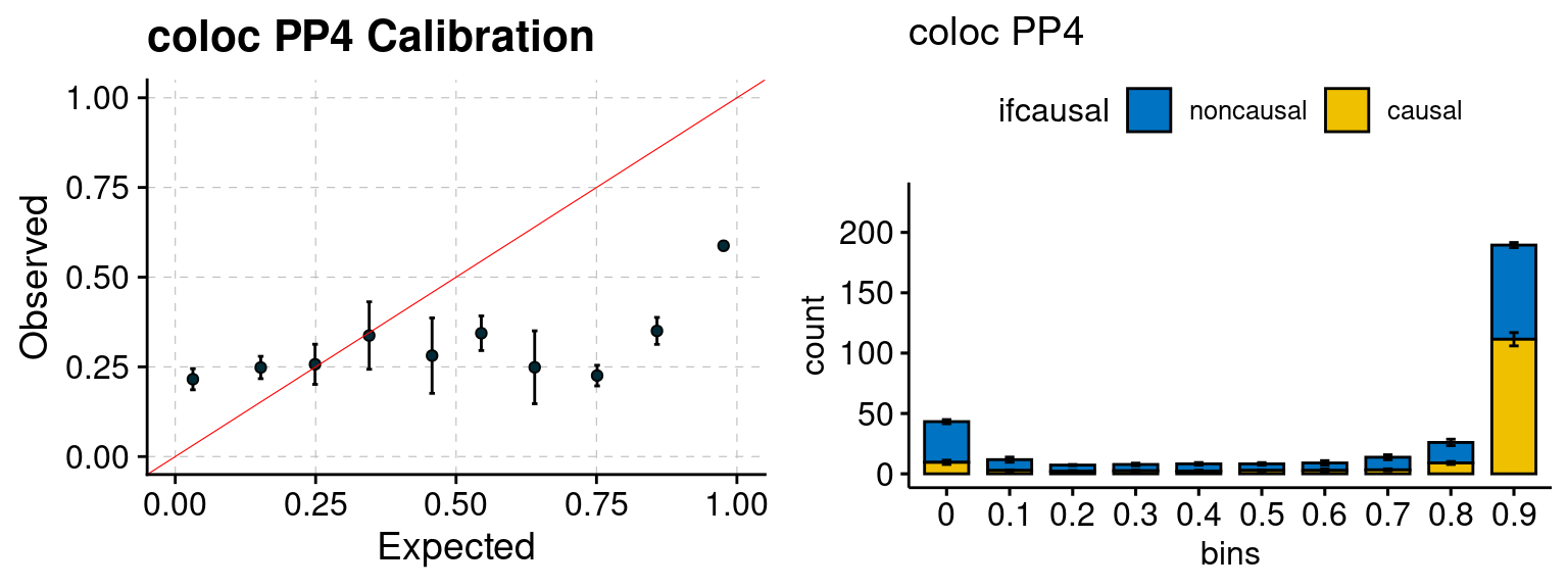
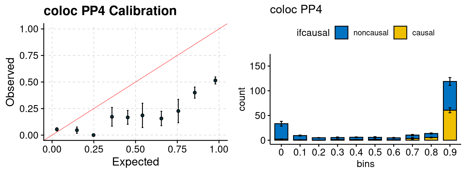
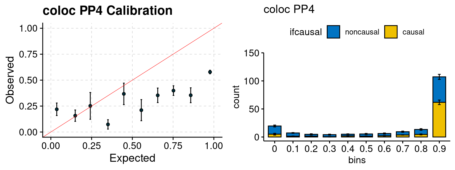
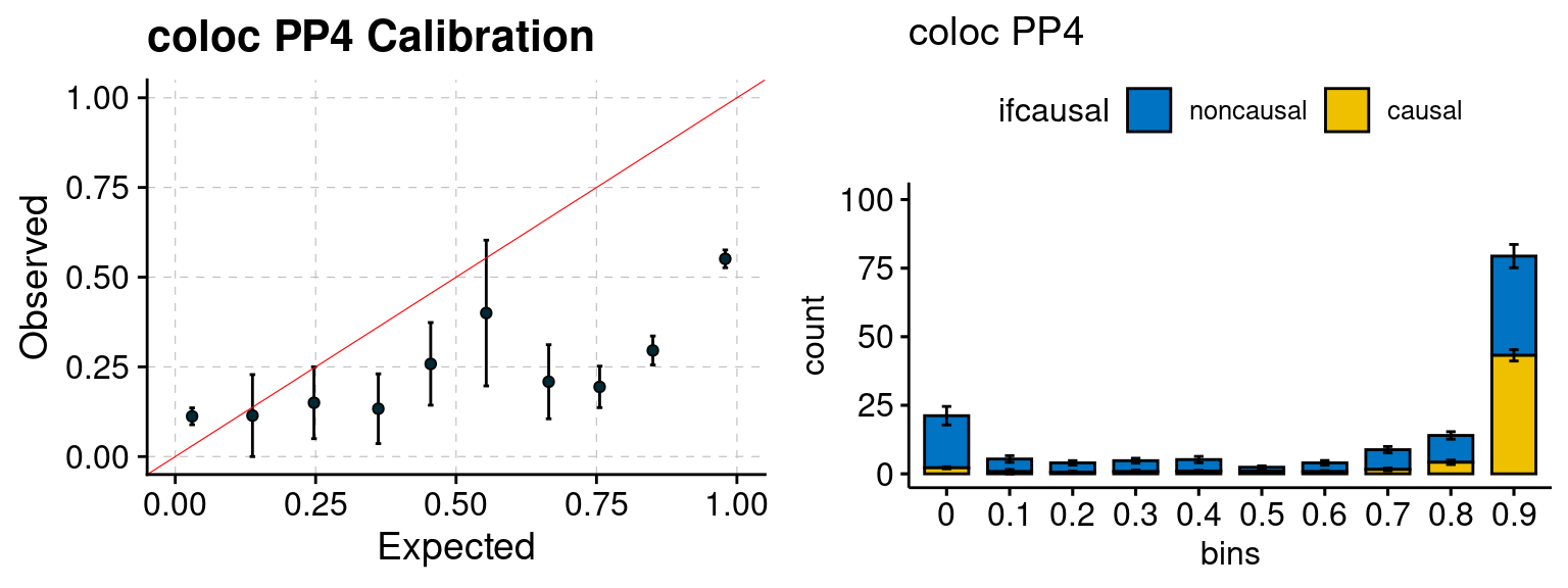
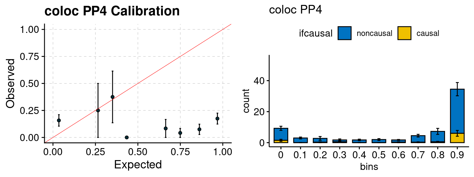
We ran coloc for all genes with TWAS p < 1e-4. We use PP4 (SNP associate with both traits). We ran SMR+HEIDI, using eQTL summary statistics GTEx v.7. We filter the results by requiring p_HEIDI > 0.05. The plots are based on SMR p value adjusted by BH method to get expected FDP.
We have tried to run MR-JTI. The results have higher false postive rate than TWAS. MR-JTI requires the SNPs be pruned before the analysis. It also requires that a gene has at least 20 eQTLs. This resulted in very few genes going into the analysis. Most genes left are in polymorphism dense regions, such as the MHC regions. I ran MR-JTI for top genes in TWAS, around 30-40% of them should be real. However, only a few genes pass MR-JTI’s 20 eQTL requirements and only 1 or 2 (5%) genes are real. We are showing MR-JTI results on this page.
plot_par <- function(configtag, runtag, simutags){
  source(paste0(outputdir, "config", configtag, ".R"))
  phenofs <- paste0(outputdir, runtag, "_simu", simutags, "-pheno.Rd")
  susieIfs <- paste0(outputdir, runtag, "_simu", simutags, "_config", configtag, ".s2.susieIrssres.Rd")
  susieIfs2 <- paste0(outputdir, runtag, "_simu",simutags, "_config", configtag,".s2.susieIrss.txt")

  mtx <- show_param(phenofs, susieIfs, susieIfs2, thin = thin)
  par(mfrow=c(1,3))
  cat("simulations ", paste(simutags, sep=",") , ": ")
  cat("mean gene PVE:", mean(mtx[, "PVE.gene_truth"]), ",", "mean SNP PVE:", mean(mtx[, "PVE.SNP_truth"]), "\n")
  plot_param(mtx)
}

plot_PIP <- function(configtag, runtag,  simutags){
   phenofs <- paste0(outputdir, "ukb-s80.45-adi", "_simu", simutags, "-pheno.Rd")
   susieIfs <- paste0(outputdir, runtag, "_simu",simutags, "_config", configtag,".susieIrss.txt")

   f1 <- caliPIP_plot(phenofs, susieIfs)
   f2 <- ncausal_plot(phenofs, susieIfs)
   gridExtra::grid.arrange(f1, f2, ncol =2)
}

plot_fusion_coloc <- function(configtag, runtag,  simutags){
    phenofs <- paste0(outputdir, runtag, "_simu", simutags, "-pheno.Rd")
    fusioncolocfs <- paste0(comparedir, runtag, "_simu", simutags, ".Adipose_Subcutaneous.coloc.result")

    f1 <- caliFUSIONp_plot(phenofs, fusioncolocfs)
    f2 <- ncausalFUSIONp_plot(phenofs, fusioncolocfs)
    f3 <- caliFUSIONbon_plot(phenofs, fusioncolocfs)
    f4 <- ncausalFUSIONbon_plot(phenofs, fusioncolocfs)
    f5 <- caliPP4_plot(phenofs, fusioncolocfs, twas.p = 0.05/J)
    f6 <- ncausalPP4_plot(phenofs, fusioncolocfs, twas.p = 0.05/J)
    gridExtra::grid.arrange(f1, f2, ncol=2)
    gridExtra::grid.arrange(f3, f4, ncol=2)
    gridExtra::grid.arrange(f5, f6, ncol=2)
}

plot_focus <- function(configtag, runtag,  simutags){
    phenofs <- paste0(outputdir, runtag, "_simu", simutags, "-pheno.Rd")
    focusfs <- paste0(comparedir, runtag, "_simu", simutags, ".Adipose_Subcutaneous.focus.tsv")

    f1 <- califocusPIP_plot(phenofs, focusfs)
    f2 <- ncausalfocusPIP_plot(phenofs, focusfs)
    gridExtra::grid.arrange(f1, f2, ncol=2)
}

plot_smr <- function(configtag, runtag,  simutags){
    phenofs <- paste0(outputdir, runtag, "_simu", simutags, "-pheno.Rd")
    smrfs <- paste0(comparedir, runtag, "_simu", simutags, ".Adipose_Subcutaneous.smr")

    f1 <- caliSMRp_plot(phenofs, smrfs)
    f2 <- ncausalSMRp_plot(phenofs, smrfs)
    gridExtra::grid.arrange(f1, f2, ncol=2)
}

plot_mrjti <- function(configtag, runtag,  simutags){
    phenofs <- paste0(outputdir, runtag, "_simu", simutags, "-pheno.Rd")
    mrfs <- paste0(comparedir, runtag, "_simu", simutags, ".Adipose_Subcutaneous.mrjti.result")

    f1 <- caliMR_plot(phenofs, mrfs)
    f2 <- ncausalMR_plot(phenofs, mrfs)
    gridExtra::grid.arrange(f1, f2, ncol=2)
}
configtag <- 1
runtag = "ukb-s80.45-adi"
simutags <- paste(1, c(1,2,5), sep = "-")
plot_par(configtag, runtag, simutags)simulations 1-1 1-2 1-5 : mean gene PVE: 0.1002441 , mean SNP PVE: 0.4907204 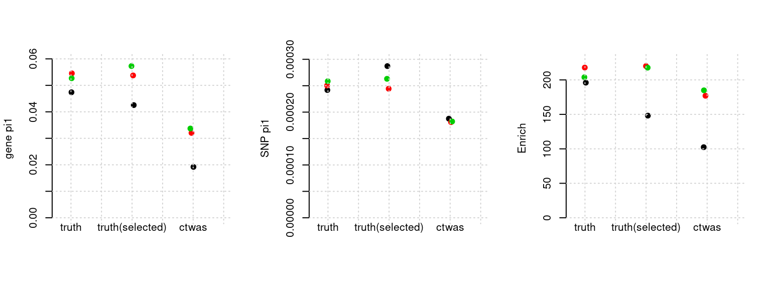
plot_PIP(configtag, runtag, simutags)
plot_fusion_coloc(configtag, runtag, simutags)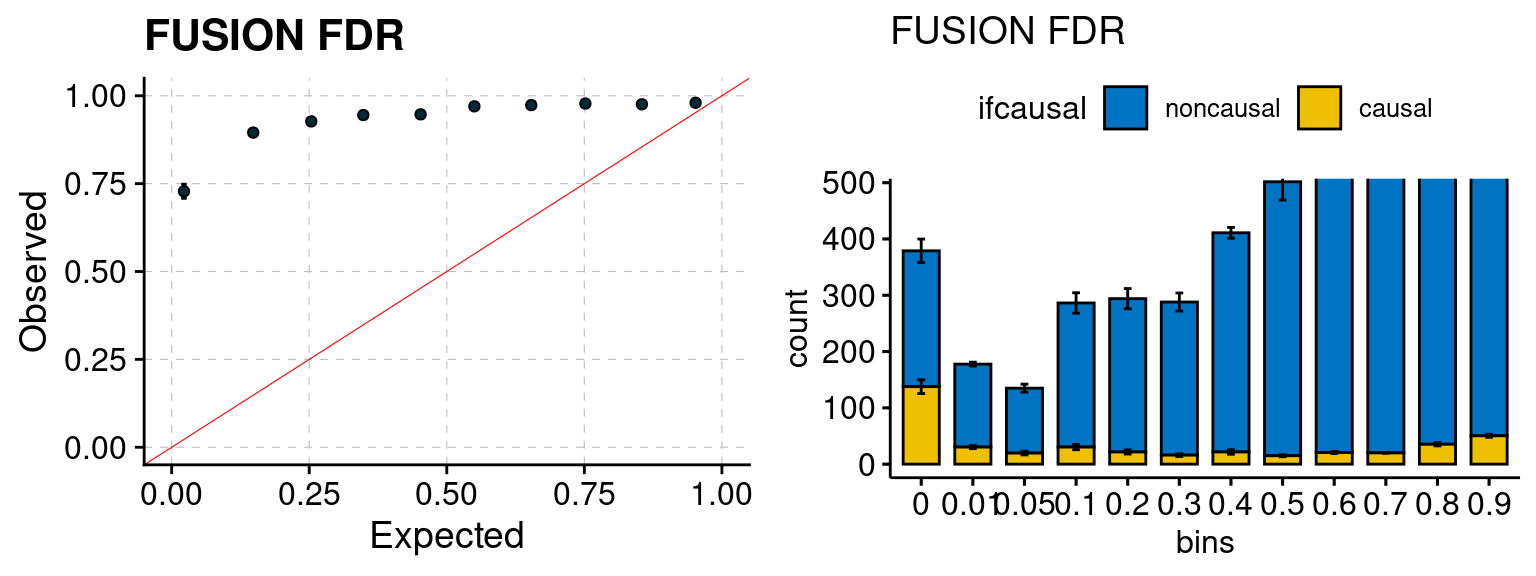
plot_focus(configtag, runtag, simutags)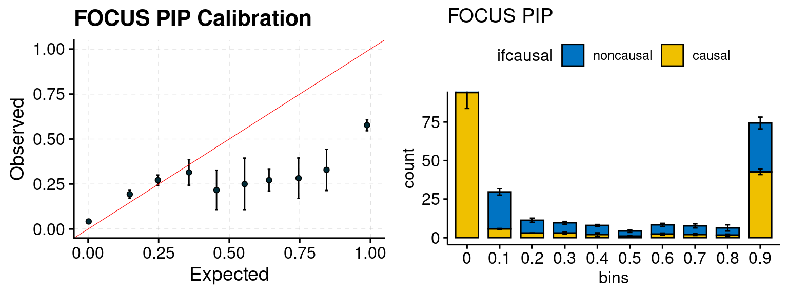
plot_smr(configtag, runtag, simutags)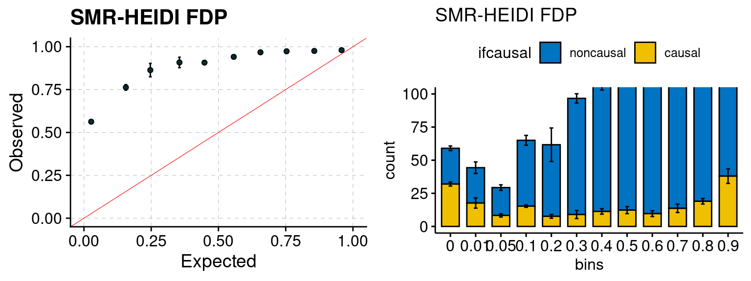
simutags <- paste(2, 1:5, sep = "-")
plot_par(configtag, runtag, simutags)
simulations 2-1 2-2 2-3 2-4 2-5 : mean gene PVE: 0.1080029 , mean SNP PVE: 0.4925448 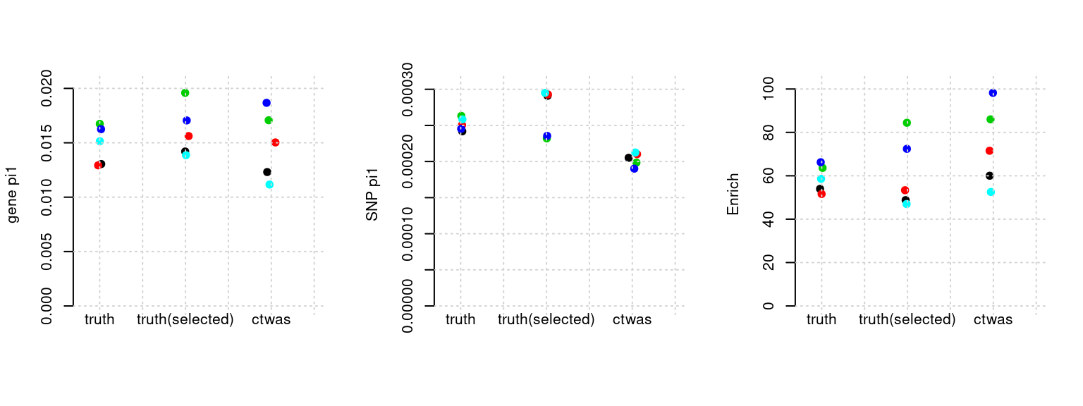
plot_PIP(configtag, runtag, simutags)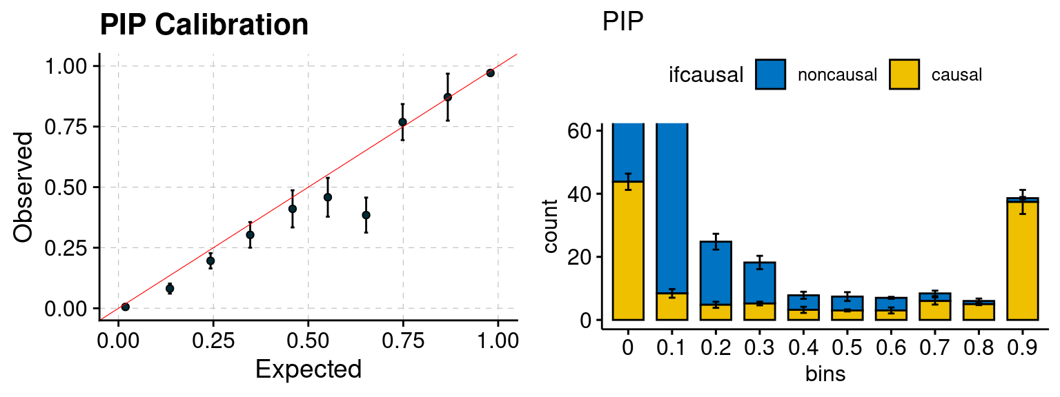
plot_fusion_coloc(configtag, runtag, simutags)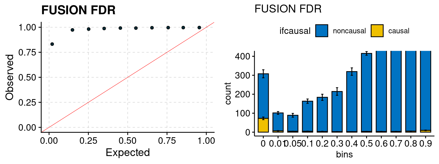
plot_focus(configtag, runtag, simutags)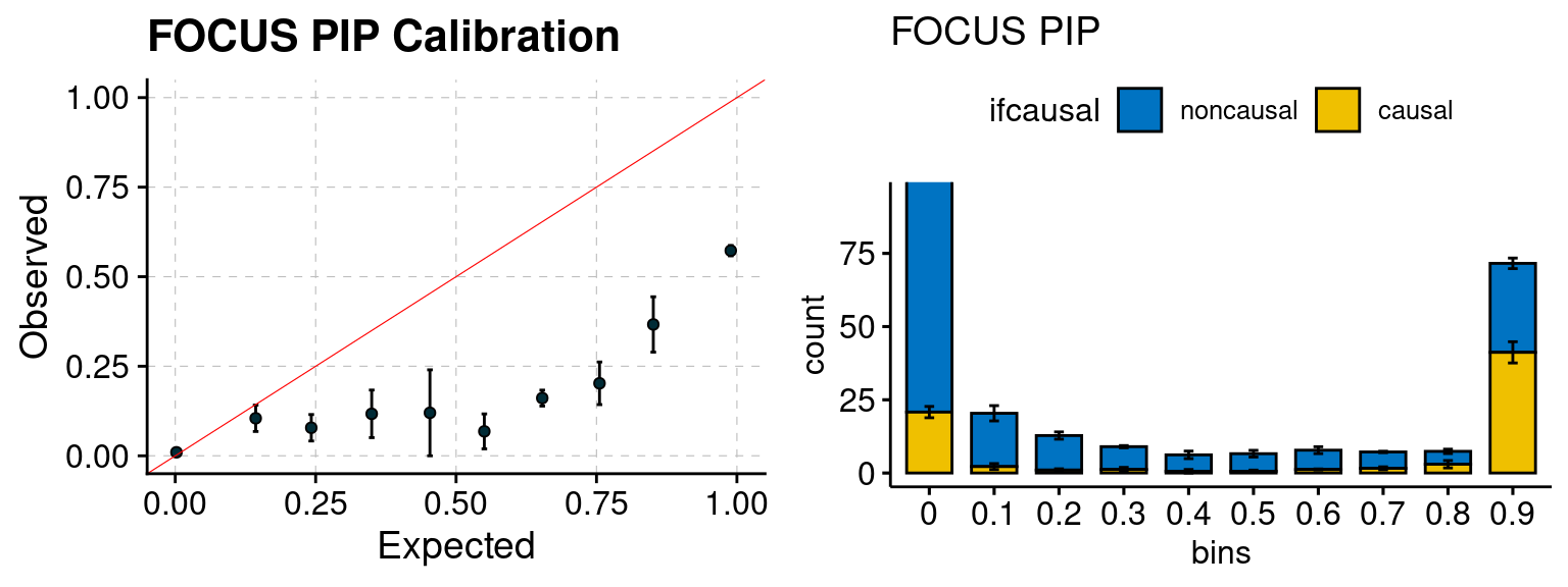
plot_smr(configtag, runtag, simutags)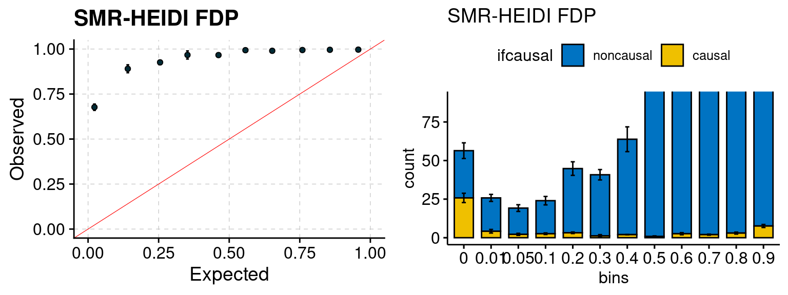
simutags <- paste(3, 1:5, sep = "-")
plot_par(configtag, runtag, simutags)
simulations 3-1 3-2 3-3 3-4 3-5 : mean gene PVE: 0.05033594 , mean SNP PVE: 0.499349 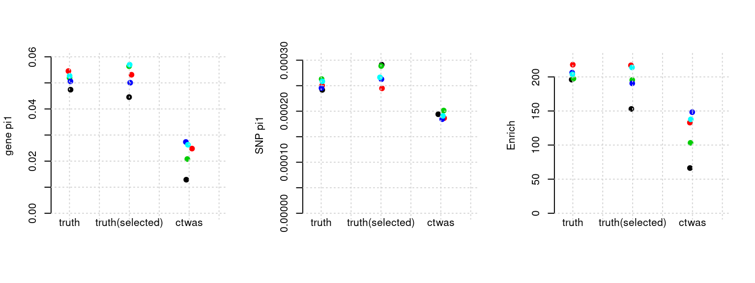
plot_PIP(configtag, runtag, simutags)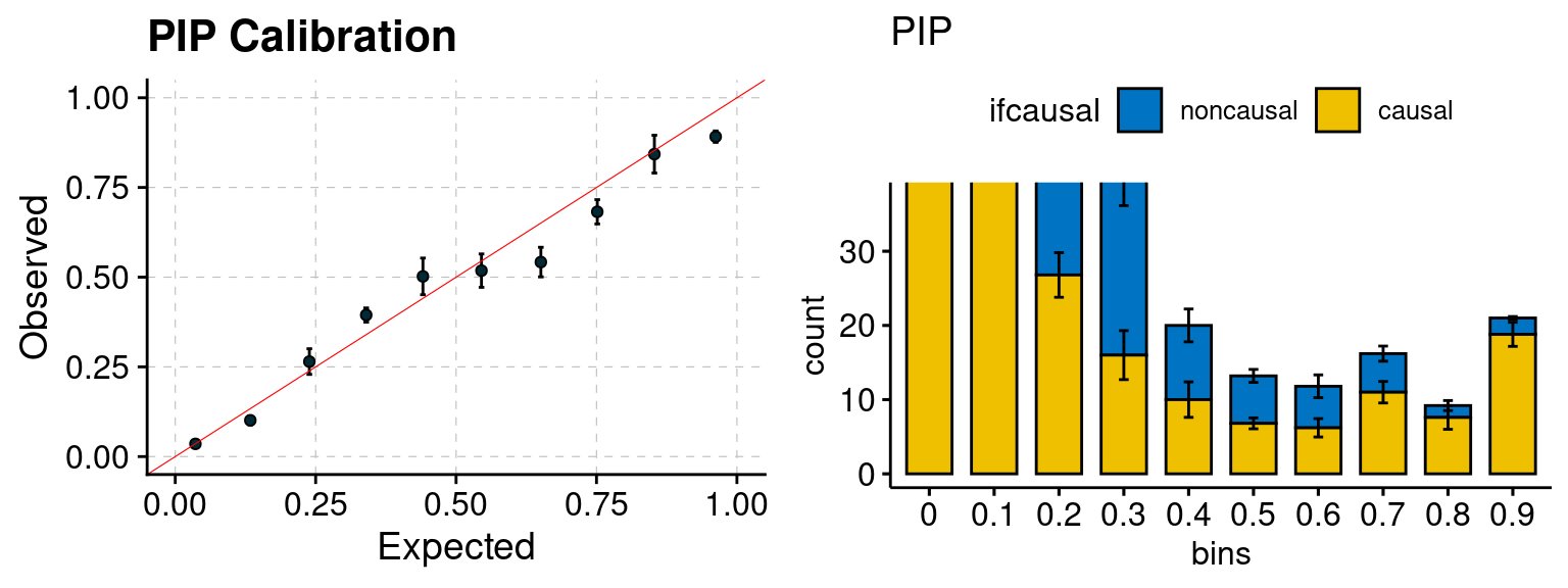
plot_fusion_coloc(configtag, runtag, simutags)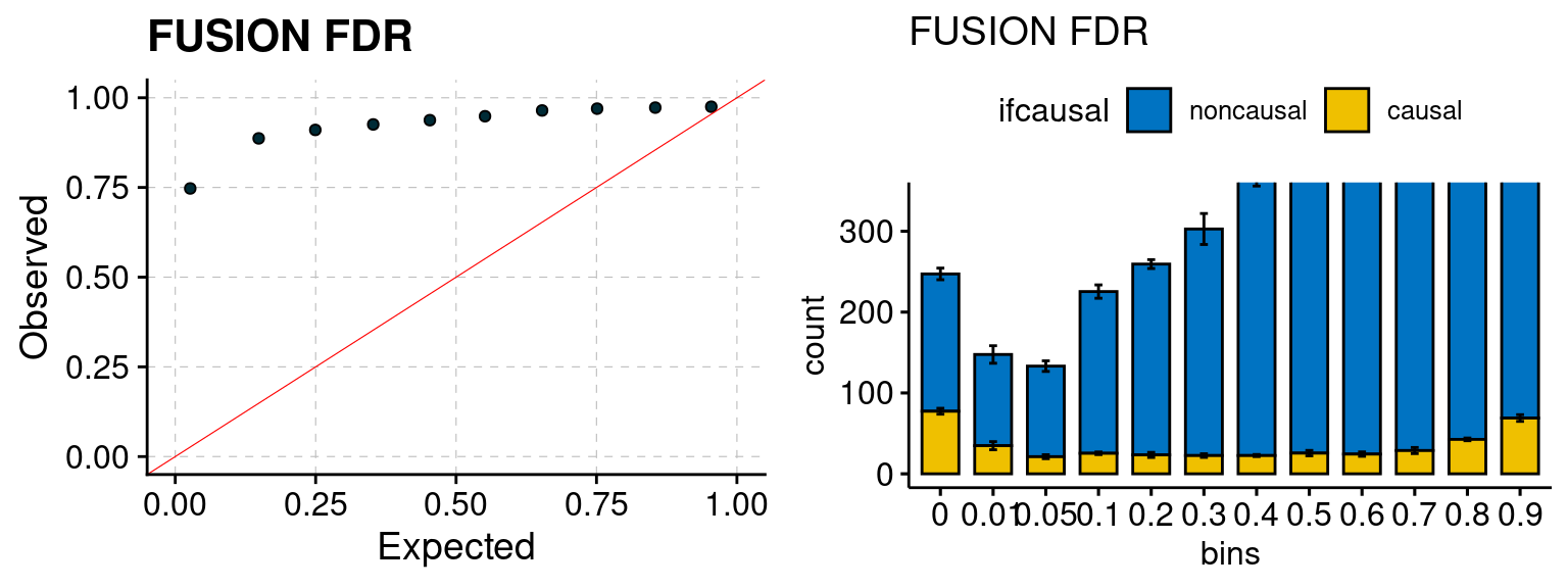
plot_focus(configtag, runtag, simutags)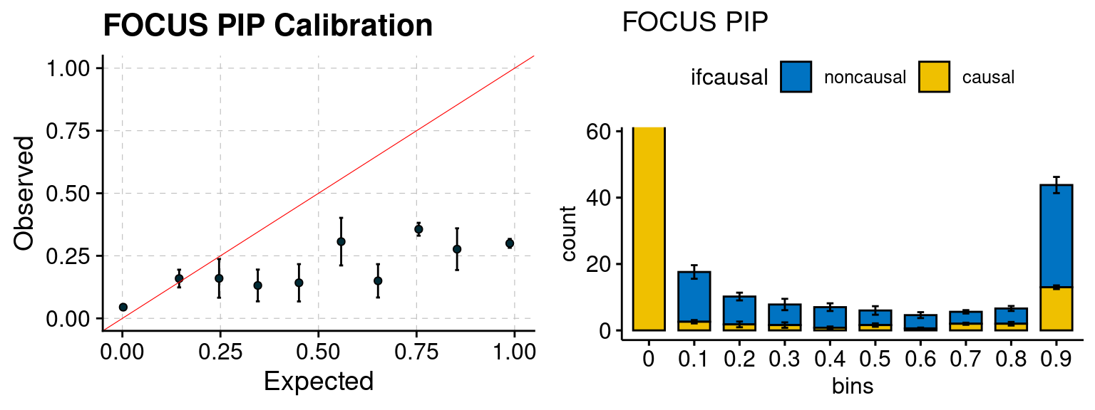
plot_smr(configtag, runtag, simutags)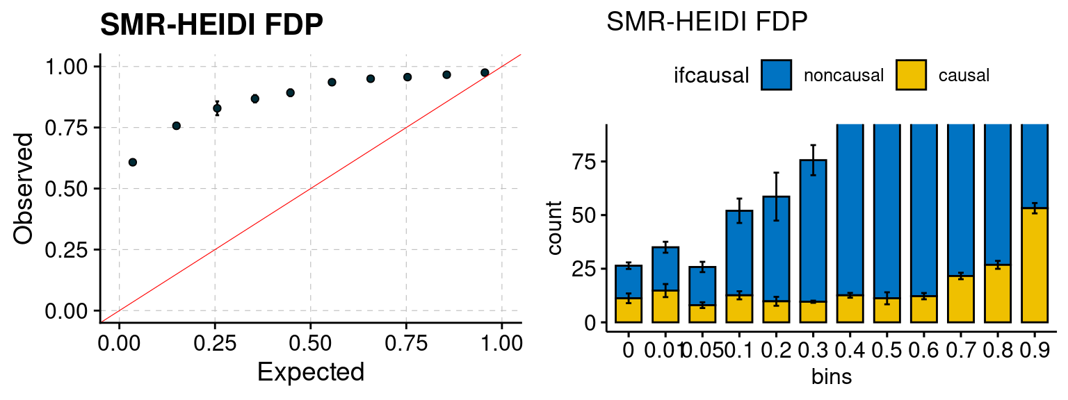
simutags <- paste(4, 1:5, sep = "-")
plot_par(configtag, runtag, simutags)
simulations 4-1 4-2 4-3 4-4 4-5 : mean gene PVE: 0.05430913 , mean SNP PVE: 0.4942206 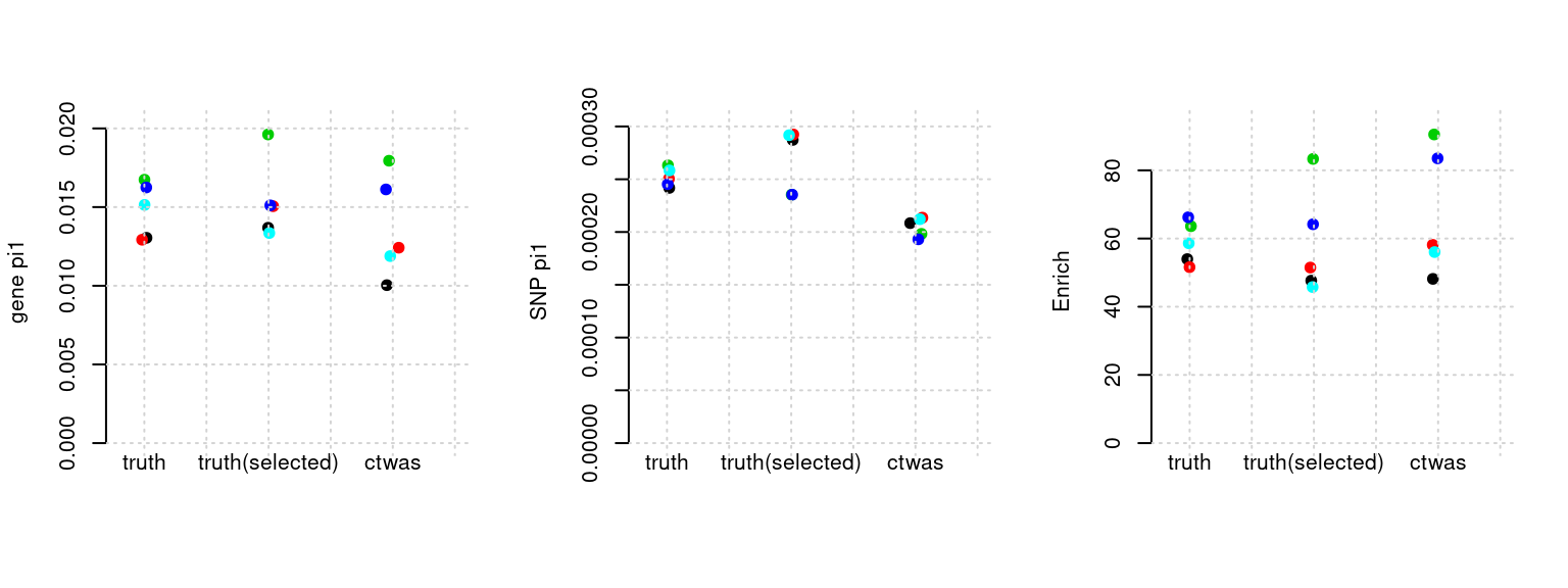
plot_PIP(configtag, runtag, simutags)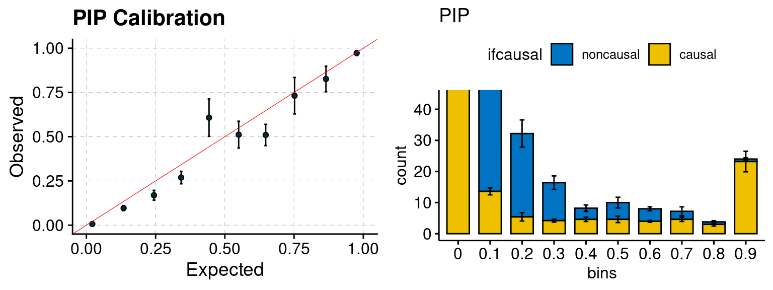
plot_fusion_coloc(configtag, runtag, simutags)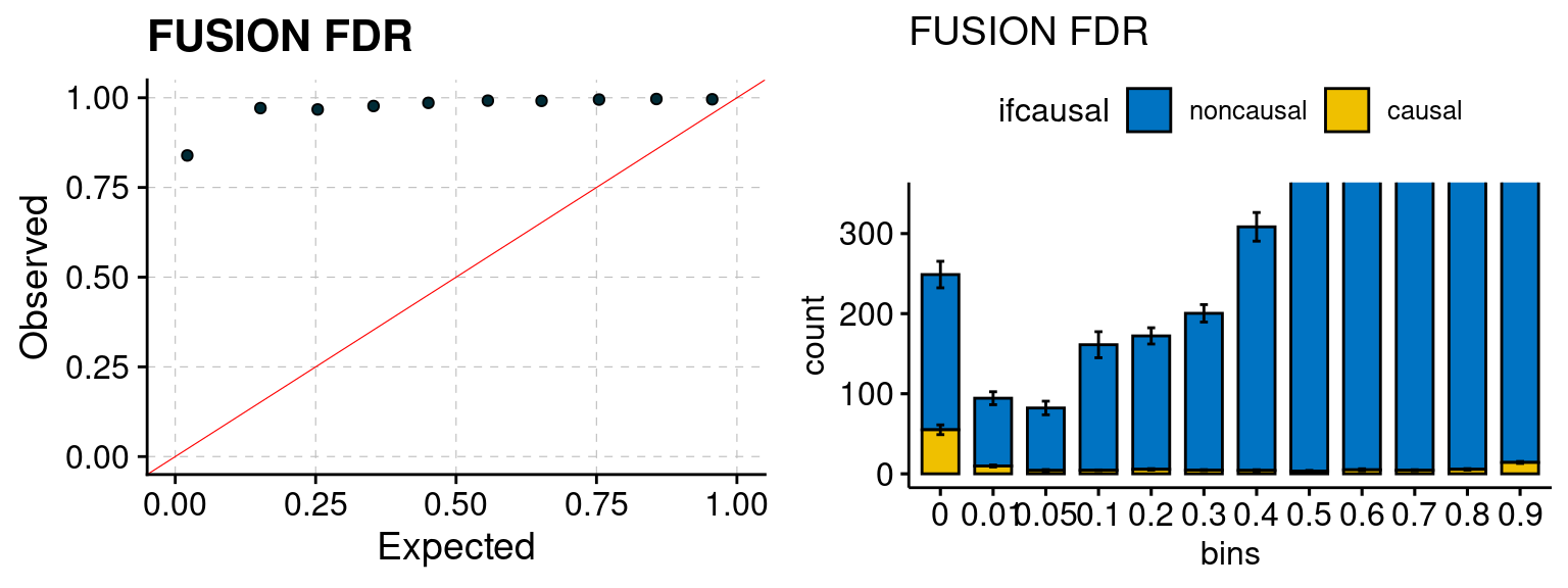
plot_focus(configtag, runtag, simutags)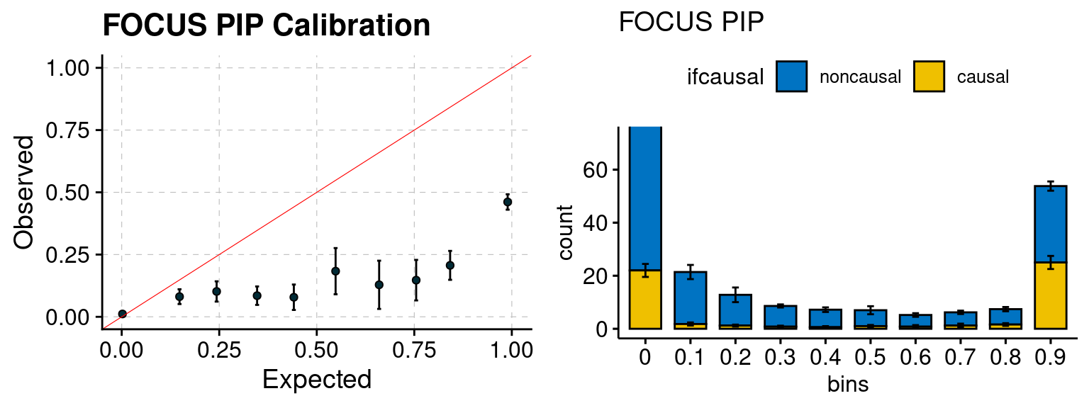
plot_smr(configtag, runtag, simutags)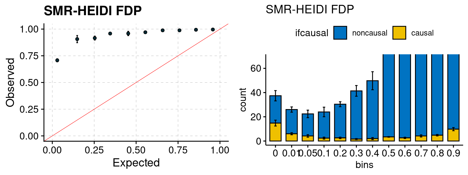
simutags <- paste(5, c(1, 3:5), sep = "-")
plot_par(configtag, runtag, simutags)
simulations 5-1 5-3 5-4 5-5 : mean gene PVE: 0.199856 , mean SNP PVE: 0.499843 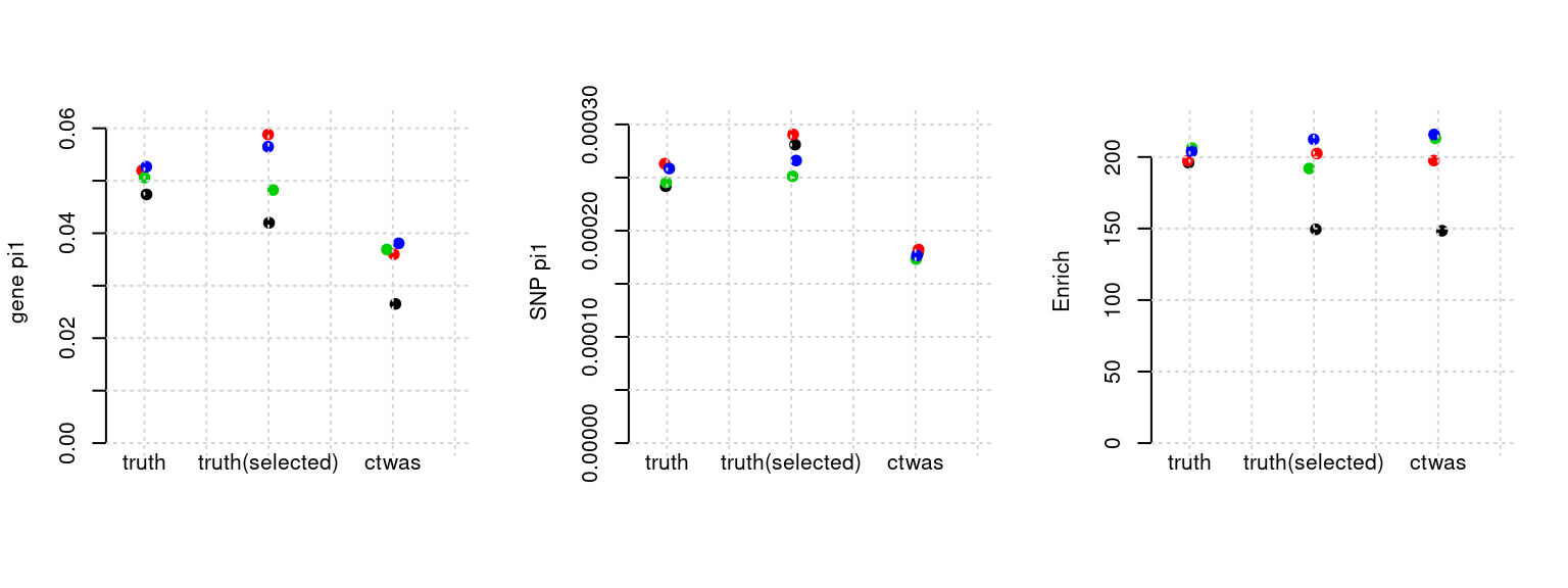
plot_PIP(configtag, runtag, simutags)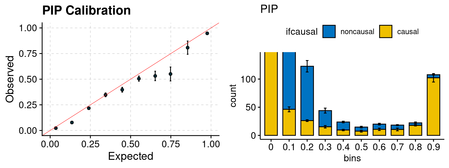
plot_fusion_coloc(configtag, runtag, simutags)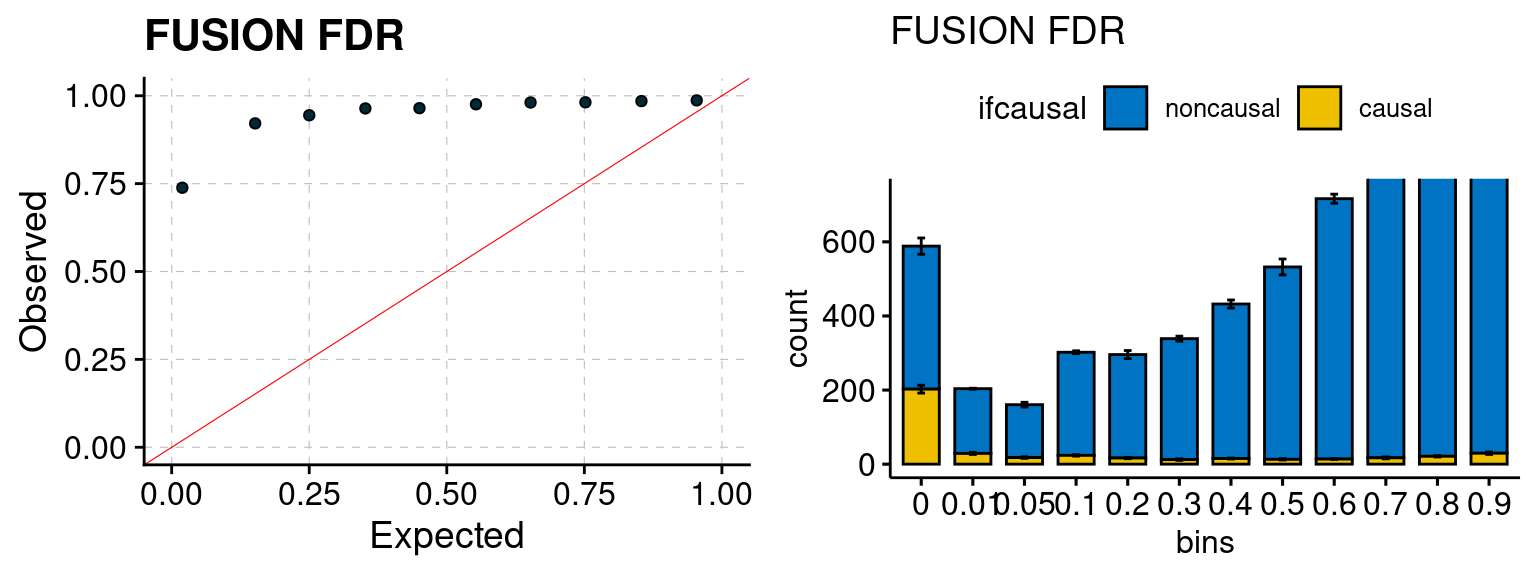
plot_focus(configtag, runtag, simutags)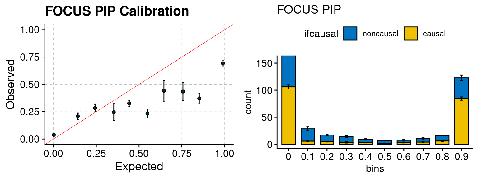
plot_smr(configtag, runtag, simutags)
simutags <- paste(6, 1:5, sep = "-")
plot_par(configtag, runtag, simutags)
simulations 6-1 6-2 6-3 6-4 6-5 : mean gene PVE: 0.2137071 , mean SNP PVE: 0.4894877 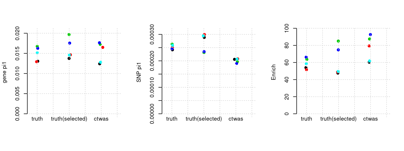
plot_PIP(configtag, runtag, simutags)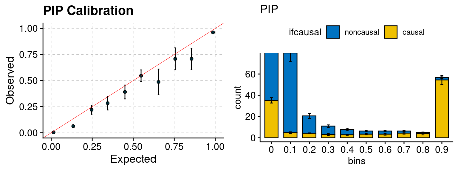
plot_fusion_coloc(configtag, runtag, simutags)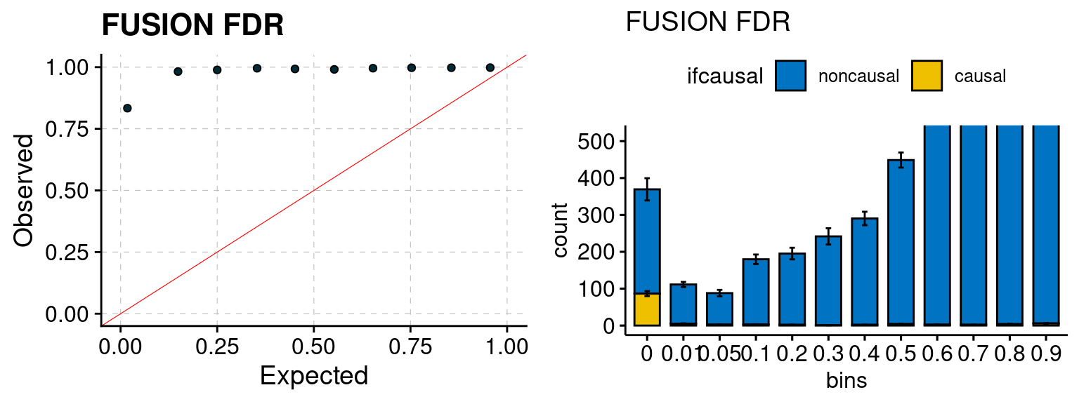
plot_focus(configtag, runtag, simutags)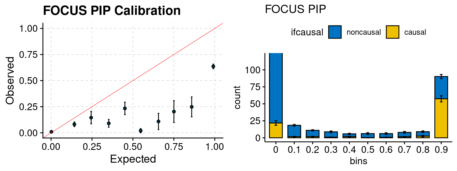
plot_smr(configtag, runtag, simutags)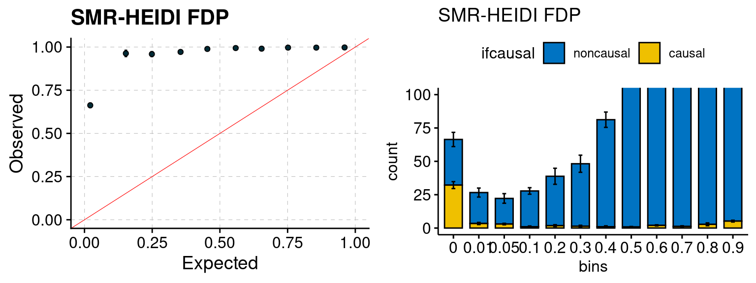
simutags <- paste(7, 1:5, sep = "-")
plot_par(configtag, runtag, simutags)
simulations 7-1 7-2 7-3 7-4 7-5 : mean gene PVE: 0.100911 , mean SNP PVE: 0.3086954 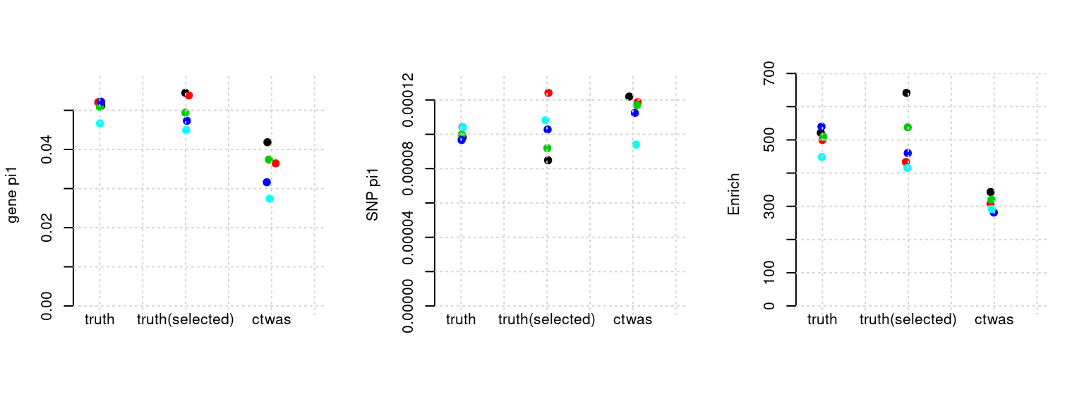
plot_PIP(configtag, runtag, simutags)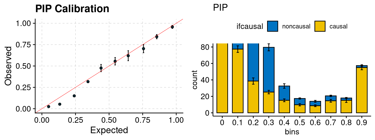
plot_fusion_coloc(configtag, runtag, simutags)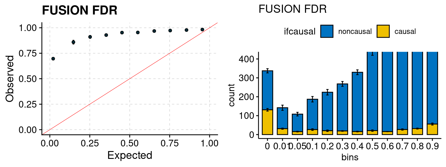
plot_focus(configtag, runtag, simutags)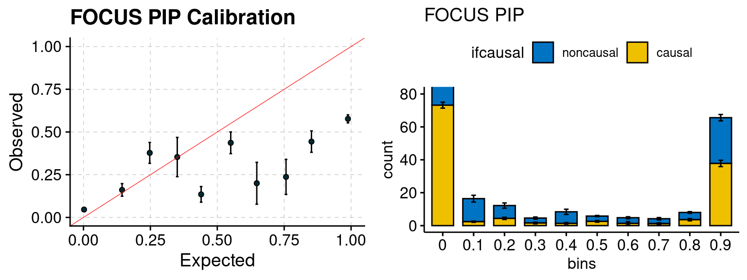
plot_smr(configtag, runtag, simutags)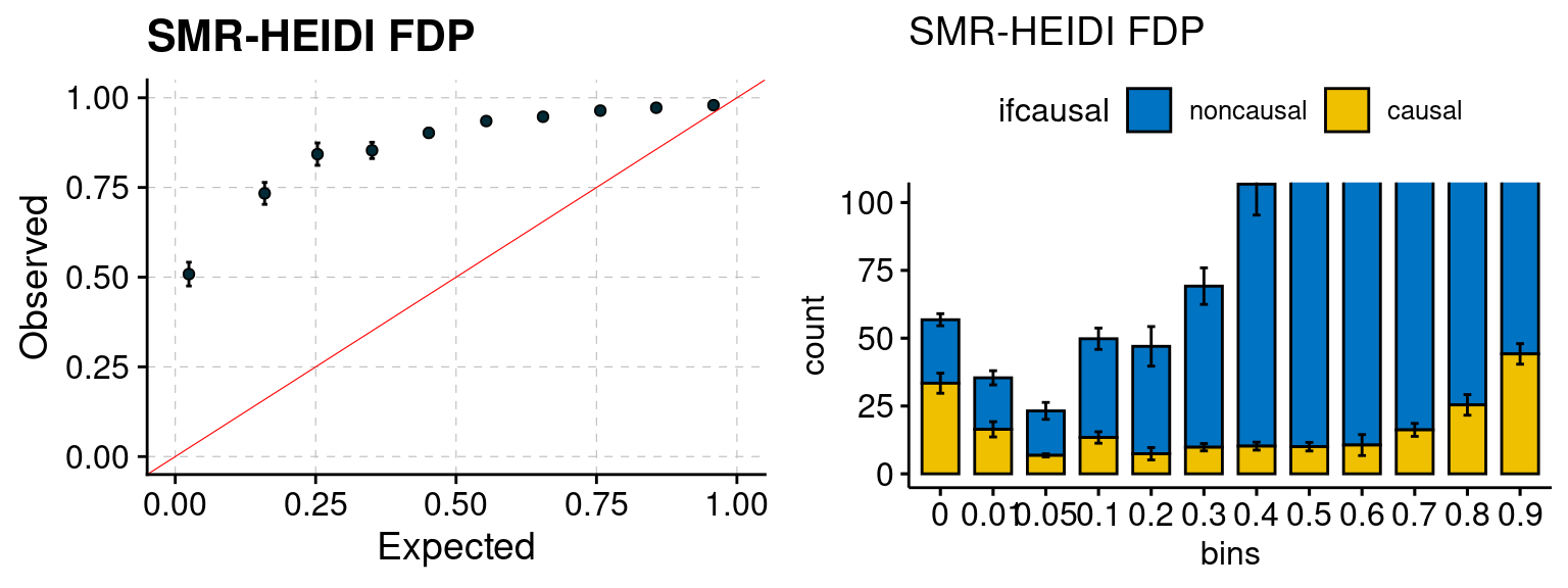
simutags <- paste(8, 1:5, sep = "-")
plot_par(configtag, runtag, simutags)
simulations 8-1 8-2 8-3 8-4 8-5 : mean gene PVE: 0.09848733 , mean SNP PVE: 0.3015623 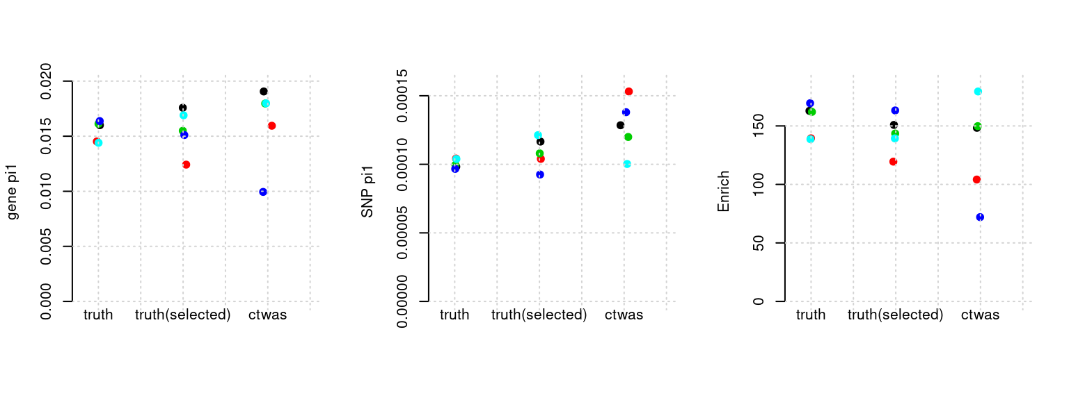
plot_PIP(configtag, runtag, simutags)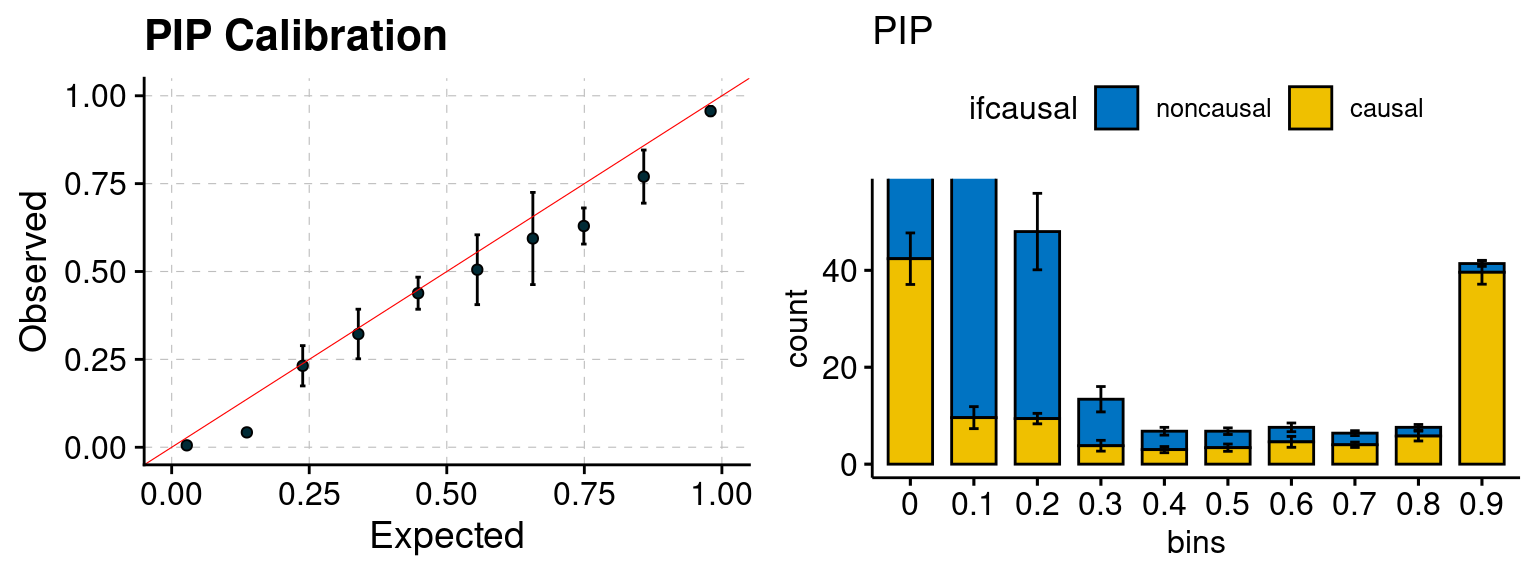
plot_fusion_coloc(configtag, runtag, simutags)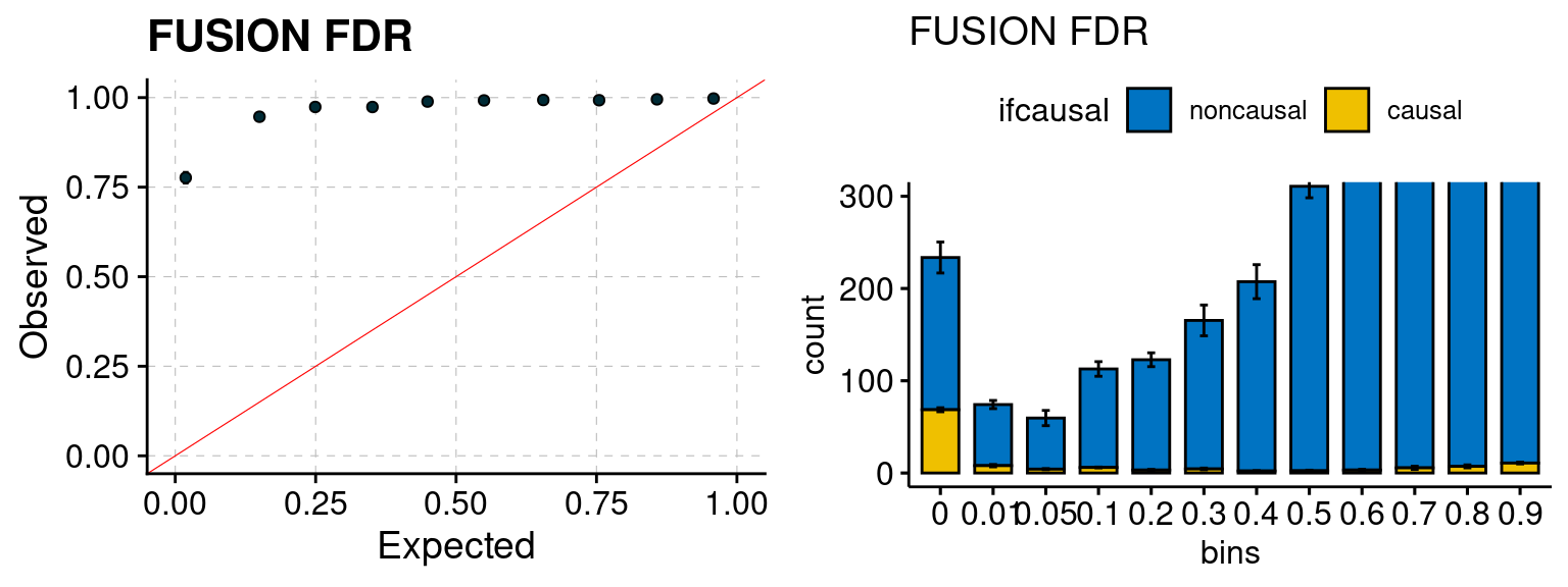
plot_focus(configtag, runtag, simutags)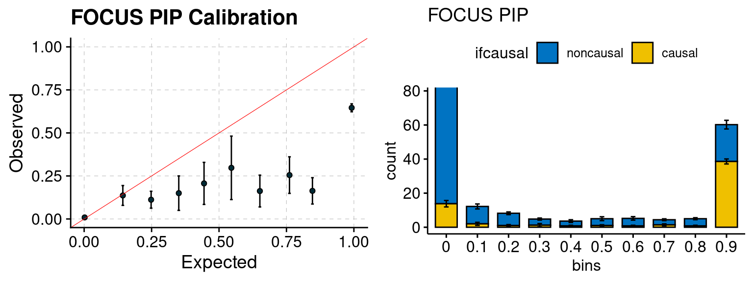
plot_smr(configtag, runtag, simutags)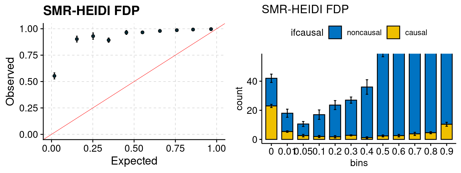
simutags <- paste(9, 1:4, sep = "-")
plot_par(configtag, runtag, simutags)
simulations 9-1 9-2 9-3 9-4 : mean gene PVE: 0.01988759 , mean SNP PVE: 0.5016792 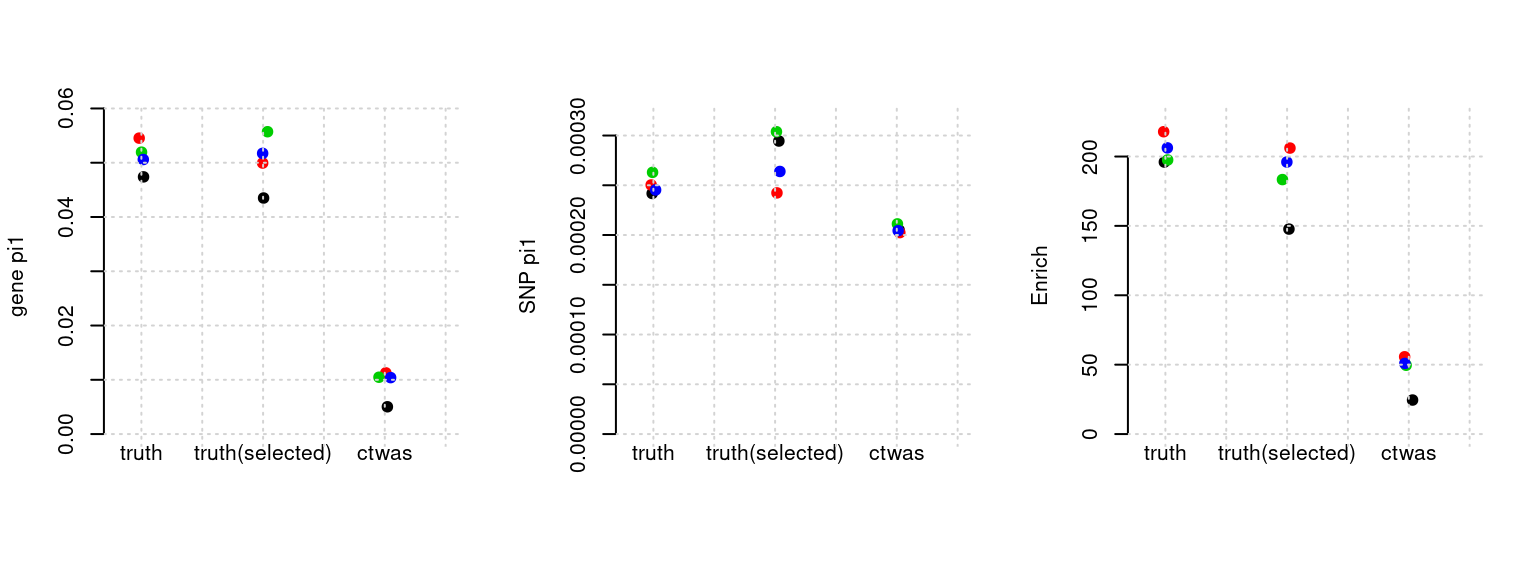
plot_PIP(configtag, runtag, simutags)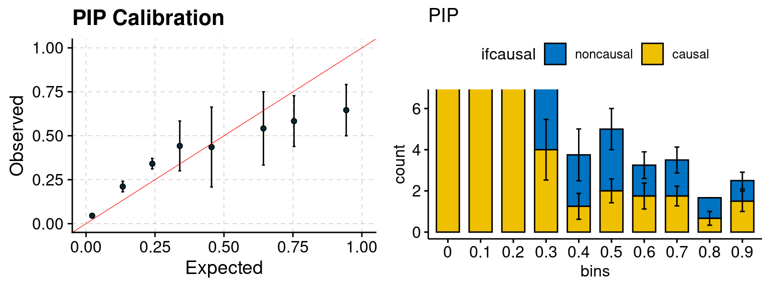
plot_fusion_coloc(configtag, runtag, simutags)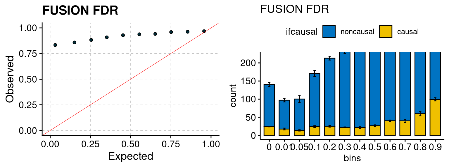
| Version | Author | Date |
|---|---|---|
| 6dee9b0 | simingz | 2021-07-22 |
plot_focus(configtag, runtag, simutags)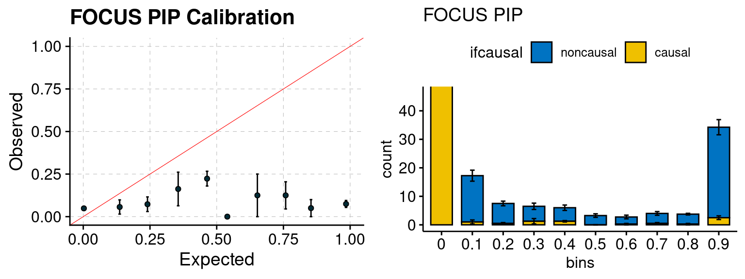
| Version | Author | Date |
|---|---|---|
| 6dee9b0 | simingz | 2021-07-22 |
plot_smr(configtag, runtag, simutags)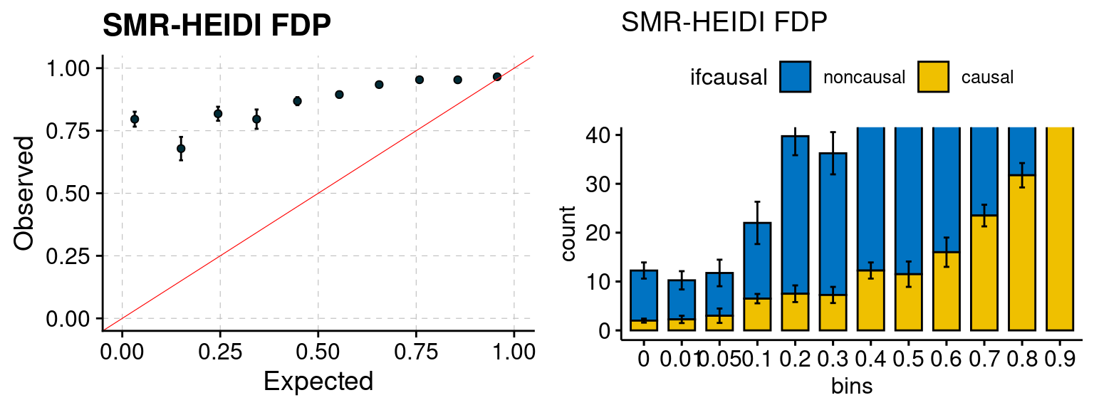
| Version | Author | Date |
|---|---|---|
| 6dee9b0 | simingz | 2021-07-22 |
simutags <- paste(10, 1:5, sep = "-")
plot_par(configtag, runtag, simutags)
simulations 10-1 10-2 10-3 10-4 10-5 : mean gene PVE: 0.02179958 , mean SNP PVE: 0.4952402 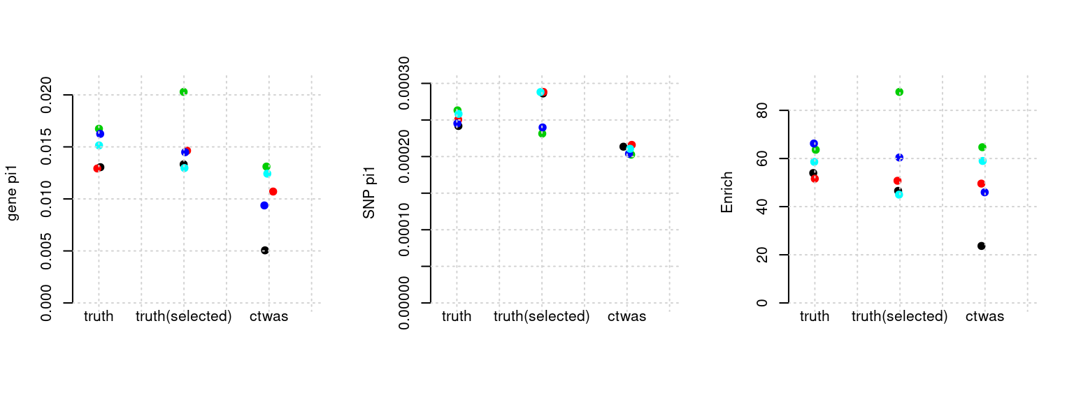
| Version | Author | Date |
|---|---|---|
| 6dee9b0 | simingz | 2021-07-22 |
plot_PIP(configtag, runtag, simutags)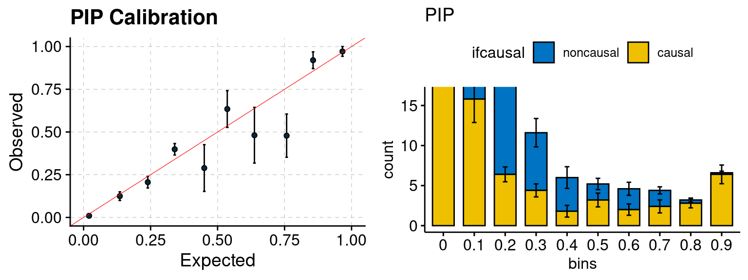
| Version | Author | Date |
|---|---|---|
| 6dee9b0 | simingz | 2021-07-22 |
plot_fusion_coloc(configtag, runtag, simutags)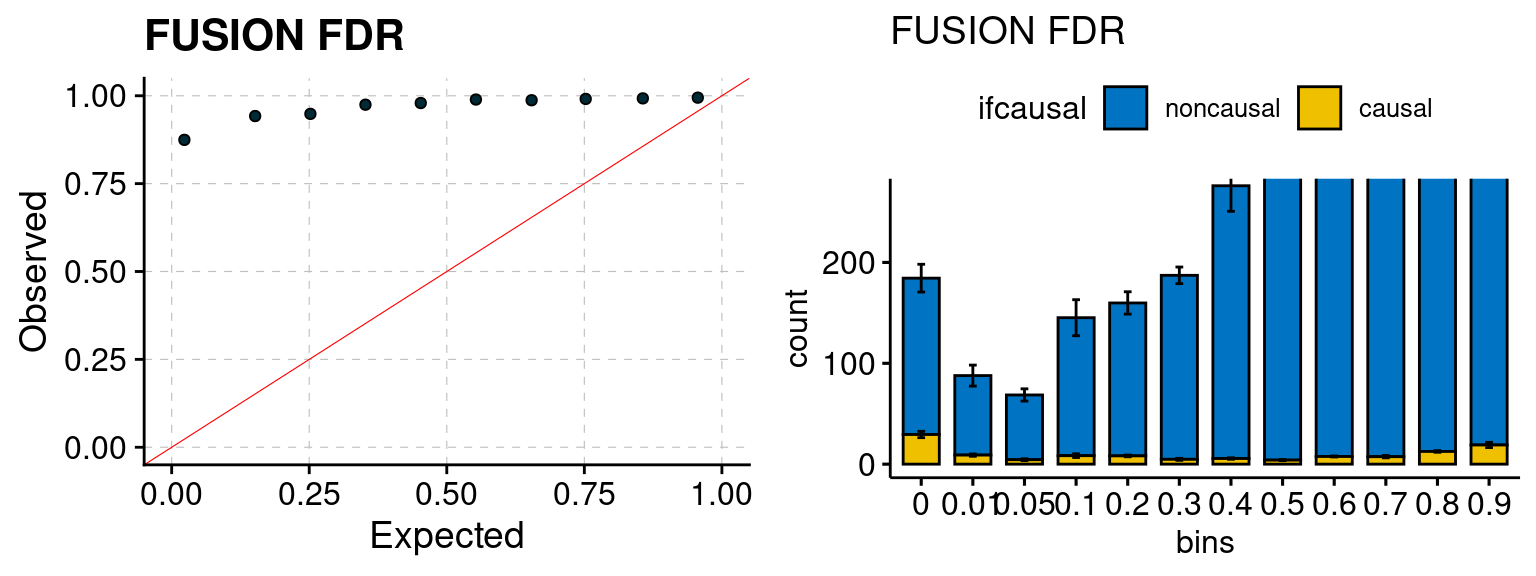
| Version | Author | Date |
|---|---|---|
| 6dee9b0 | simingz | 2021-07-22 |
| Version | Author | Date |
|---|---|---|
| 6dee9b0 | simingz | 2021-07-22 |

| Version | Author | Date |
|---|---|---|
| 6dee9b0 | simingz | 2021-07-22 |
plot_focus(configtag, runtag, simutags)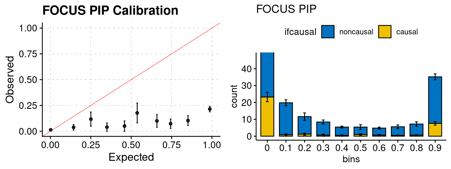
| Version | Author | Date |
|---|---|---|
| 6dee9b0 | simingz | 2021-07-22 |
plot_smr(configtag, runtag, simutags)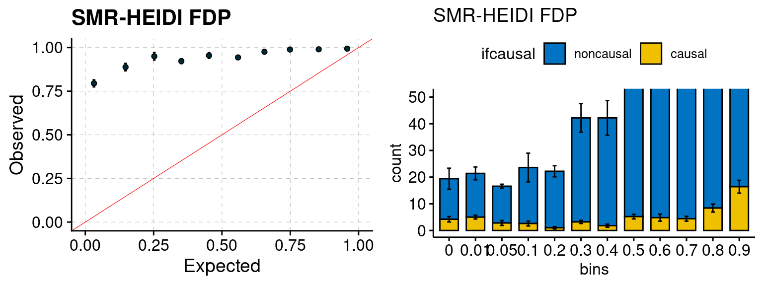
| Version | Author | Date |
|---|---|---|
| 6dee9b0 | simingz | 2021-07-22 |
ctwas results (LDR)
Using the R LD matrices as the LD reference input for ctwas, instead of the genotype type of randomly subsetted samples. The LD R matrices are generated using all 300k samples that passed the our filtering criteria (generated by Wes Crouse). A R matrice is provided for each LD block region.
configtag <- "1_LDR"
simutags <- paste(1, c(1,2,5), sep = "-")
plot_par(configtag, runtag, simutags)
simulations 1-1 1-2 1-5 : mean gene PVE: 0.1002441 , mean SNP PVE: 0.4907204 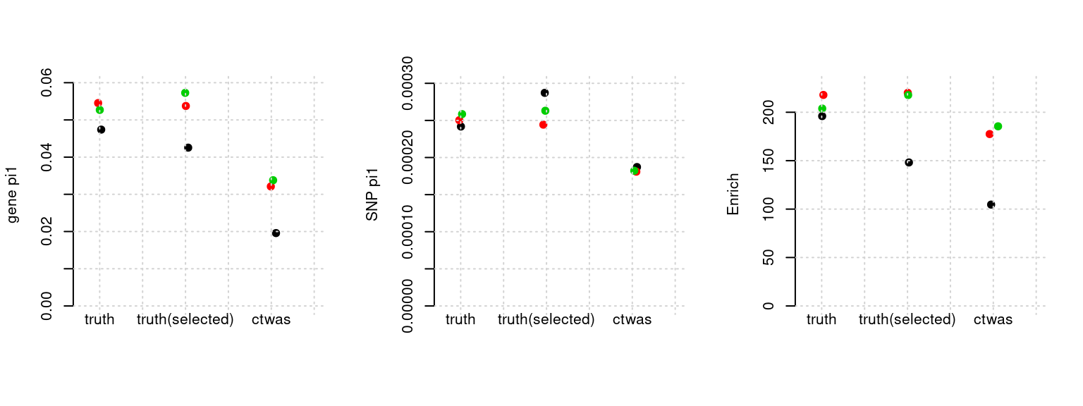
| Version | Author | Date |
|---|---|---|
| 6dee9b0 | simingz | 2021-07-22 |
plot_PIP(configtag, runtag, simutags)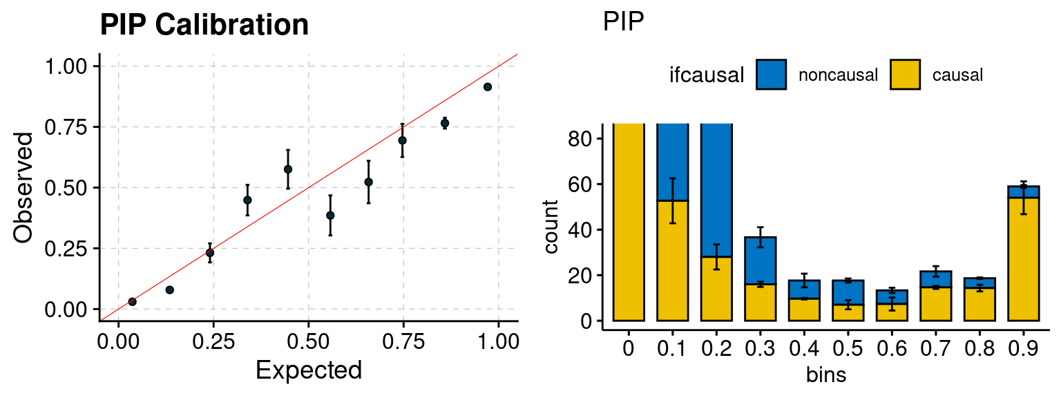
| Version | Author | Date |
|---|---|---|
| 6dee9b0 | simingz | 2021-07-22 |
simutags <- paste(2, 1:5, sep = "-")
plot_par(configtag, runtag, simutags)
simulations 2-1 2-2 2-3 2-4 2-5 : mean gene PVE: 0.1080029 , mean SNP PVE: 0.4925448 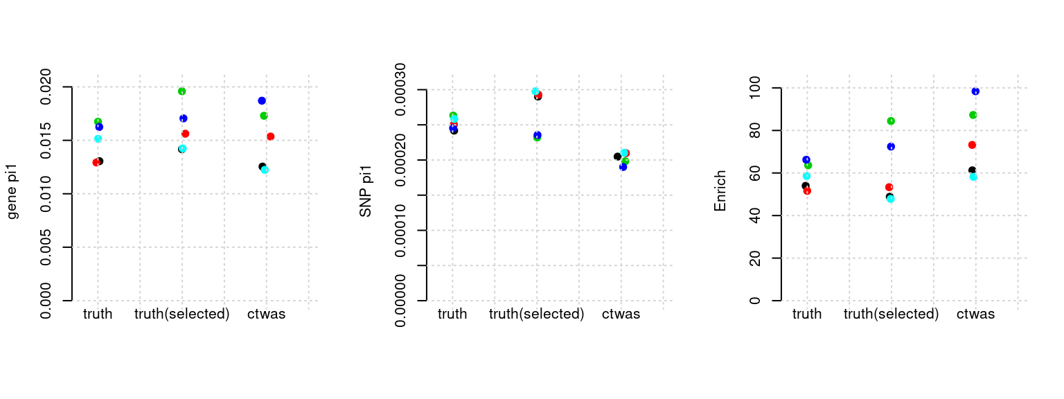
| Version | Author | Date |
|---|---|---|
| 6dee9b0 | simingz | 2021-07-22 |
plot_PIP(configtag, runtag, simutags)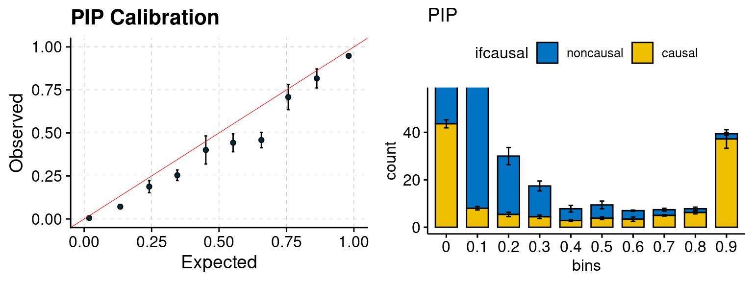
| Version | Author | Date |
|---|---|---|
| 6dee9b0 | simingz | 2021-07-22 |
simutags <- paste(3, 1:5, sep = "-")
plot_par(configtag, runtag, simutags)
simulations 3-1 3-2 3-3 3-4 3-5 : mean gene PVE: 0.05033594 , mean SNP PVE: 0.499349 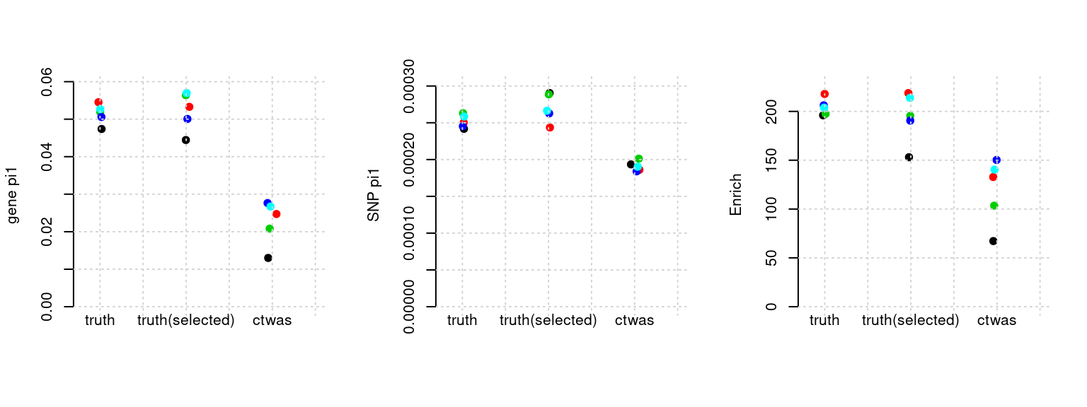
| Version | Author | Date |
|---|---|---|
| 6dee9b0 | simingz | 2021-07-22 |
plot_PIP(configtag, runtag, simutags)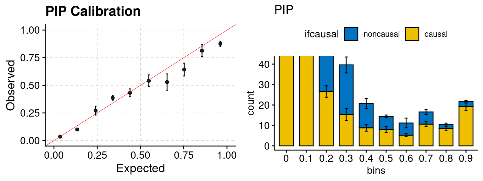
| Version | Author | Date |
|---|---|---|
| 6dee9b0 | simingz | 2021-07-22 |
simutags <- paste(4, 1:5, sep = "-")
plot_par(configtag, runtag, simutags)
simulations 4-1 4-2 4-3 4-4 4-5 : mean gene PVE: 0.05430913 , mean SNP PVE: 0.4942206 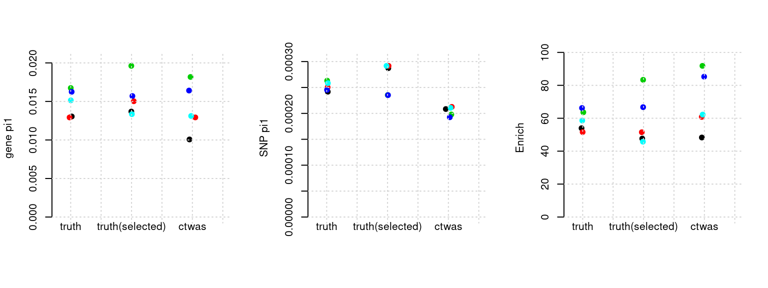
| Version | Author | Date |
|---|---|---|
| 6dee9b0 | simingz | 2021-07-22 |
plot_PIP(configtag, runtag, simutags)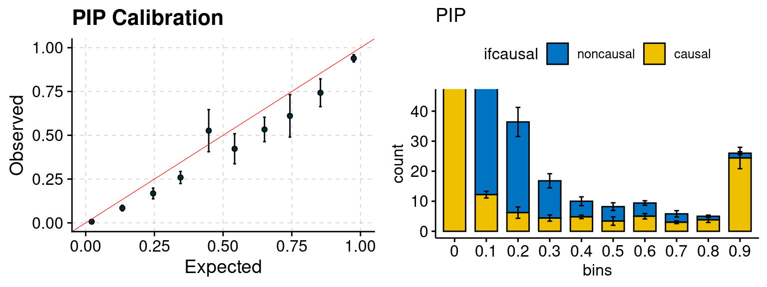
| Version | Author | Date |
|---|---|---|
| 6dee9b0 | simingz | 2021-07-22 |
sessionInfo()R version 3.6.1 (2019-07-05)
Platform: x86_64-pc-linux-gnu (64-bit)
Running under: Scientific Linux 7.4 (Nitrogen)
Matrix products: default
BLAS/LAPACK: /software/openblas-0.2.19-el7-x86_64/lib/libopenblas_haswellp-r0.2.19.so
locale:
[1] LC_CTYPE=en_US.UTF-8 LC_NUMERIC=C
[3] LC_TIME=en_US.UTF-8 LC_COLLATE=en_US.UTF-8
[5] LC_MONETARY=en_US.UTF-8 LC_MESSAGES=en_US.UTF-8
[7] LC_PAPER=en_US.UTF-8 LC_NAME=C
[9] LC_ADDRESS=C LC_TELEPHONE=C
[11] LC_MEASUREMENT=en_US.UTF-8 LC_IDENTIFICATION=C
attached base packages:
[1] stats graphics grDevices utils datasets methods base
other attached packages:
[1] ggpubr_0.4.0 plotrix_3.7-6 cowplot_1.0.0 stringr_1.4.0
[5] plyr_1.8.4 tidyr_1.1.0 plotly_4.9.0 ggplot2_3.3.3
[9] data.table_1.13.2 ctwas_0.1.28
loaded via a namespace (and not attached):
[1] httr_1.4.2 jsonlite_1.6 viridisLite_0.3.0 foreach_1.4.4
[5] R.utils_2.9.0 pgenlibr_0.2 carData_3.0-2 logging_0.10-108
[9] highr_0.8 cellranger_1.1.0 yaml_2.2.0 pillar_1.5.1
[13] backports_1.1.4 lattice_0.20-38 glue_1.4.2 digest_0.6.20
[17] promises_1.0.1 ggsignif_0.5.0 colorspace_1.4-1 R.oo_1.22.0
[21] htmltools_0.3.6 httpuv_1.6.1 Matrix_1.2-18 pkgconfig_2.0.2
[25] broom_0.7.5 haven_2.3.1 purrr_0.3.4 scales_1.1.0
[29] whisker_0.3-2 openxlsx_4.1.0.1 later_0.8.0 rio_0.5.16
[33] git2r_0.26.1 tibble_3.1.0 farver_2.1.0 generics_0.0.2
[37] car_3.0-5 ellipsis_0.2.0.1 withr_2.4.1 lazyeval_0.2.2
[41] magrittr_1.5 crayon_1.3.4 readxl_1.3.1 evaluate_0.14
[45] R.methodsS3_1.7.1 fs_1.3.1 fansi_0.4.0 rstatix_0.7.0
[49] forcats_0.4.0 foreign_0.8-71 tools_3.6.1 hms_0.5.3
[53] lifecycle_1.0.0 munsell_0.5.0 ggsci_2.9 zip_2.0.3
[57] compiler_3.6.1 rlang_0.4.10 debugme_1.1.0 grid_3.6.1
[61] iterators_1.0.10 htmlwidgets_1.3 labeling_0.3 rmarkdown_2.9
[65] gtable_0.3.0 codetools_0.2-16 abind_1.4-5 DBI_1.1.0
[69] curl_3.3 R6_2.4.0 gridExtra_2.3 knitr_1.33
[73] dplyr_1.0.5 utf8_1.1.4 workflowr_1.6.2 rprojroot_1.3-2
[77] stringi_1.4.3 Rcpp_1.0.5 vctrs_0.3.7 tidyselect_1.1.0
[81] xfun_0.24