Last updated: 2023-06-10

Checks: 5 2

Knit directory: causal-TWAS/

This reproducible R Markdown analysis was created with workflowr (version 1.6.2). The Checks tab describes the reproducibility checks that were applied when the results were created. The Past versions tab lists the development history.

R Markdown file: uncommitted changes

The R Markdown file has unstaged changes. To know which version of the R Markdown file created these results, you’ll want to first commit it to the Git repo. If you’re still working on the analysis, you can ignore this warning. When you’re finished, you can run wflow_publish to commit the R Markdown file and build the HTML.

Environment: empty

Great job! The global environment was empty. Objects defined in the global environment can affect the analysis in your R Markdown file in unknown ways. For reproduciblity it’s best to always run the code in an empty environment.

Seed: set.seed(20191103)

The command set.seed(20191103) was run prior to running the code in the R Markdown file. Setting a seed ensures that any results that rely on randomness, e.g. subsampling or permutations, are reproducible.

Session information: recorded

Great job! Recording the operating system, R version, and package versions is critical for reproducibility.

Cache: none

Nice! There were no cached chunks for this analysis, so you can be confident that you successfully produced the results during this run.

File paths: absolute

Using absolute paths to the files within your workflowr project makes it difficult for you and others to run your code on a different machine. Change the absolute path(s) below to the suggested relative path(s) to make your code more reproducible.

absolute	relative
~/causalTWAS/causal-TWAS/analysis/summarize_ctwas_plots.R	analysis/summarize_ctwas_plots.R
~/causalTWAS/causal-TWAS/analysis/summarize_twas-coloc_plots.R	analysis/summarize_twas-coloc_plots.R
~/causalTWAS/causal-TWAS/analysis/summarize_focus_plots.R	analysis/summarize_focus_plots.R
~/causalTWAS/causal-TWAS/analysis/summarize_smr_plots.R	analysis/summarize_smr_plots.R
~/causalTWAS/causal-TWAS/analysis/summarize_mrjti_plots.R	analysis/summarize_mrjti_plots.R
~/causalTWAS/causal-TWAS/code/qqplot.R	code/qqplot.R

Repository version: 3631063

Great! You are using Git for version control. Tracking code development and connecting the code version to the results is critical for reproducibility.

The results in this page were generated with repository version 3631063. See the Past versions tab to see a history of the changes made to the R Markdown and HTML files.

Note that you need to be careful to ensure that all relevant files for the analysis have been committed to Git prior to generating the results (you can use wflow_publish or wflow_git_commit). workflowr only checks the R Markdown file, but you know if there are other scripts or data files that it depends on. Below is the status of the Git repository when the results were generated:


Ignored files:
    Ignored:    .Rhistory
    Ignored:    .Rproj.user/
    Ignored:    .ipynb_checkpoints/
    Ignored:    analysis/.ipynb_checkpoints/
    Ignored:    code/.ipynb_checkpoints/
    Ignored:    code/before_package/.ipynb_checkpoints/
    Ignored:    code/workflow/.ipynb_checkpoints/
    Ignored:    code/workflow/.snakemake/
    Ignored:    code/workflow/logs/.snakemake/
    Ignored:    data/
    Ignored:    output/.ipynb_checkpoints/

Unstaged changes:
    Modified:   analysis/index.Rmd
    Modified:   analysis/simulation-ctwas-ukbWG-gtex.adipose_s80.45_03222023.Rmd
    Modified:   code/run_ctwas_rss2.R
    Modified:   code/workflow/Snakefile-simu_20230321
    Modified:   code/workflow/Snakefile-simu_20230322

Note that any generated files, e.g. HTML, png, CSS, etc., are not included in this status report because it is ok for generated content to have uncommitted changes.

These are the previous versions of the repository in which changes were made to the R Markdown (analysis/simulation-ctwas-ukbWG-gtex.adipose_s80.45_03222023.Rmd) and HTML (docs/simulation-ctwas-ukbWG-gtex.adipose_s80.45_03222023.html) files. If you’ve configured a remote Git repository (see ?wflow_git_remote), click on the hyperlinks in the table below to view the files as they were in that past version.

File	Version	Author	Date	Message
Rmd	3631063	simingz	2023-06-05	remove L=1 results for low PVE
html	3631063	simingz	2023-06-05	remove L=1 results for low PVE
Rmd	972fe6d	simingz	2023-06-05	low PVE simulation bug fix
html	972fe6d	simingz	2023-06-05	low PVE simulation bug fix
Rmd	a08d87e	simingz	2023-05-25	PVEgene=0.02
html	a08d87e	simingz	2023-05-25	PVEgene=0.02
html	9a1264b	simingz	2023-05-10	L=1 for ctwas rerun of 45k
Rmd	f260f7d	simingz	2023-05-10	L=1 for ctwas rerun of 113k
Rmd	de95a10	simingz	2023-05-08	110k simulation
html	de95a10	simingz	2023-05-08	110k simulation
Rmd	d76d5c4	simingz	2023-04-20	more simulation settings for low SNP PVE
html	d76d5c4	simingz	2023-04-20	more simulation settings for low SNP PVE

library(ctwas)
library(data.table)
suppressMessages({library(plotly)})
library(tidyr)
library(plyr)
library(stringr)
source("~/causalTWAS/causal-TWAS/analysis/summarize_ctwas_plots.R")
source('~/causalTWAS/causal-TWAS/analysis/summarize_twas-coloc_plots.R')
source('~/causalTWAS/causal-TWAS/analysis/summarize_focus_plots.R')
source('~/causalTWAS/causal-TWAS/analysis/summarize_smr_plots.R')
source('~/causalTWAS/causal-TWAS/analysis/summarize_mrjti_plots.R')
source('~/causalTWAS/causal-TWAS/code/qqplot.R')

pgenfn = "/home/simingz/causalTWAS/ukbiobank/ukb_pgen_s80.45/ukb-s80.45_pgenfs.txt"
ld_pgenfn = "/home/simingz/causalTWAS/ukbiobank/ukb_pgen_s80.45/ukb-s80.45.2_pgenfs.txt"
outputdir = "/home/simingz/causalTWAS/simulations/simulation_ctwas_rss_20230322/" # /
comparedir = "/home/simingz/causalTWAS/simulations/simulation_ctwas_rss_20230322_compare/"
runtag = "ukb-s80.45-adi"

simutags = paste(rep(1:9, each = length(1:5)), 1:5, sep = "-")

pgenfs <- read.table(pgenfn, header = F, stringsAsFactors = F)[,1]
pvarfs <- sapply(pgenfs, prep_pvar, outputdir = outputdir)

ld_pgenfs <- read.table(ld_pgenfn, header = F, stringsAsFactors = F)[,1]
ld_pvarfs <- sapply(ld_pgenfs, prep_pvar, outputdir = outputdir)

pgens <- lapply(1:length(pgenfs), function(x) prep_pgen(pgenf = pgenfs[x],pvarf = pvarfs[x]))

Analysis description

n.ori <- 80000 # number of samples
n <- pgenlibr::GetRawSampleCt(pgens[[1]])
p <- sum(unlist(lapply(pgens, pgenlibr::GetVariantCt))) # number of SNPs
J <- 8021 # number of genes

Data

The same as 20210416. We tried a few additional settings with small SNP heritablity (0.2) or large gene heritablity (0.5) following the suggestions by reviewers.

Analysis

ctwas

Get z scores for gene expression. We used expression models and LD reference to get z scores for gene expression.
Run ctwas_rss ctwas_rss algorithm first runs on all regions to get rough estimate for gene and SNP prior. Then run on small regions (having small probablities of having > 1 causal signals based on rough estimates) to get more accurate estimate. To lower computational burden, we downsampled SNPs (0.1) to estimate parameters. With the estimated parameters, we then run susie for all regions using both genes and downsampled SNPs with specified \(L\). After this, for regions with strong gene signals, we rerun susie with full SNPs using specified \(L\).

Configurations

ld_regions ='EUR', We used LDetect to define regions. To match UKbiobank data, we use the ‘EUR’ population

thin = 0.1, downsampled SNPs to 1/10 for parameter estimation step

niter1 =3, run niter1 =3 iterations first to get some rough parameter estimates.

prob_single = 0.8, the probability of a region having at most 1 singal has to be at least 0.8 to be selected for the parameter estimation step. This probability is obtained by using the PIPs from the first few iterations.

niter2 = 30, run niter2 = 30 for parameter estimation step

group_prior = NULL, the initiating prior parameters we used for running susie for each region is uniform prior for genes and SNPs.

group_prior_var = NULL, the initiating prior variance parameters we used for running susie for each region follows susie_rss’s default (50).

max_SNP_region = 5000, the maximum number of SNPs for re-running susie on strong gene signal regions is 5000.

We have two configurations for L: config 1 the last step of ctwas was running susie with L=5 in regions with big gene PIPs, config 2 the last step of ctwas was running susie with L=1 in regions with big gene PIPs.

`ctwas` results

Results: Each row shows parameter estimation results from 20 simulation runs with similar settings (i.e. pi1 and PVE for genes and SNPs). Results from each run were represented by one dot, dots with the same color come from the same run. truth: the true parameters, selected_truth: the truth in selected regions that were used to estimate parameters, ctwas: ctwas estimated parameters (using summary statistics as input).

Note, we have three configurations, config1, config2, config3. Config 1 was run with wrong harmonziation configuration, they were rerun the last step as config3. This were run by v.0.1.29 (harmonize_z = F for config3, harmonize_z = T for config1.)

plot_par <- function(configtag, runtag, simutags){
  source(paste0(outputdir, "config", configtag, ".R"))
  phenofs <- paste0(outputdir, runtag, "_simu", simutags, "-pheno.Rd")
  susieIfs <- paste0(outputdir, runtag, "_simu", simutags, "_config", configtag, ".s2.susieIrssres.Rd")
  susieIfs2 <- paste0(outputdir, runtag, "_simu",simutags, "_config", configtag,".s2.susieIrss.txt")

  mtx <- show_param(phenofs, susieIfs, susieIfs2, thin = thin)
  par(mfrow=c(1,3))
  cat("simulations ", paste(simutags, sep=",") , ": ")
  cat("mean gene PVE:", mean(mtx[, "PVE.gene_truth"]), ",", "mean SNP PVE:", mean(mtx[, "PVE.SNP_truth"]), "\n")
  plot_param(mtx)
}

plot_PIP <- function(configtag, runtag,  simutags){
   phenofs <- paste0(outputdir, "ukb-s80.45-adi", "_simu", simutags, "-pheno.Rd")
   susieIfs <- paste0(outputdir, runtag, "_simu",simutags, "_config", configtag,".susieIrss.txt")

   f1 <- caliPIP_plot(phenofs, susieIfs)
   f2 <- ncausal_plot(phenofs, susieIfs) 
   gridExtra::grid.arrange(f1, f2, ncol =2)
}

plot_fusion_coloc <- function(configtag, runtag,  simutags){
    phenofs <- paste0(outputdir, runtag, "_simu", simutags, "-pheno.Rd")
    fusioncolocfs <- paste0(comparedir, runtag, "_simu", simutags, ".Adipose_Subcutaneous.coloc.result")
    
    f1 <- caliFUSIONp_plot(phenofs, fusioncolocfs)
    f2 <- ncausalFUSIONp_plot(phenofs, fusioncolocfs)
    f3 <- caliFUSIONbon_plot(phenofs, fusioncolocfs)
    f4 <- ncausalFUSIONbon_plot(phenofs, fusioncolocfs)
    f5 <- caliPP4_plot(phenofs, fusioncolocfs, twas.p = 0.05/J)
    f6 <- ncausalPP4_plot(phenofs, fusioncolocfs, twas.p = 0.05/J)
    gridExtra::grid.arrange(f1, f2, ncol=2)
    gridExtra::grid.arrange(f3, f4, ncol=2)
    gridExtra::grid.arrange(f5, f6, ncol=2)
}
    
plot_focus <- function(configtag, runtag,  simutags){
    phenofs <- paste0(outputdir, runtag, "_simu", simutags, "-pheno.Rd")
    focusfs <- paste0(comparedir, runtag, "_simu", simutags, ".Adipose_Subcutaneous.focus.tsv")
    
    f1 <- califocusPIP_plot(phenofs, focusfs)
    f2 <- ncausalfocusPIP_plot(phenofs, focusfs)
    gridExtra::grid.arrange(f1, f2, ncol=2)
}

plot_smr <- function(configtag, runtag,  simutags){
    phenofs <- paste0(outputdir, runtag, "_simu", simutags, "-pheno.Rd")
    smrfs <- paste0(comparedir, runtag, "_simu", simutags, ".Adipose_Subcutaneous.smr")
    
    f1 <- caliSMRp_plot(phenofs, smrfs)
    f2 <- ncausalSMRp_plot(phenofs, smrfs)
    gridExtra::grid.arrange(f1, f2, ncol=2)
}

plot_mrjti <- function(configtag, runtag,  simutags){
    phenofs <- paste0(outputdir, runtag, "_simu", simutags, "-pheno.Rd")
    mrfs <- paste0(comparedir, runtag, "_simu", simutags, ".Adipose_Subcutaneous.mrjti.result")
    
    f1 <- caliMR_plot(phenofs, mrfs)
    f2 <- ncausalMR_plot(phenofs, mrfs)
    gridExtra::grid.arrange(f1, f2, ncol=2)
}

#configtag <- 1
runtag = "ukb-s80.45-adi"

simutags <- paste(1, c(1:5), sep = "-")
plot_par(1, runtag, simutags)

simulations  1-1 1-2 1-3 1-4 1-5 : mean gene PVE: 0.010832 , mean SNP PVE: 0.09835368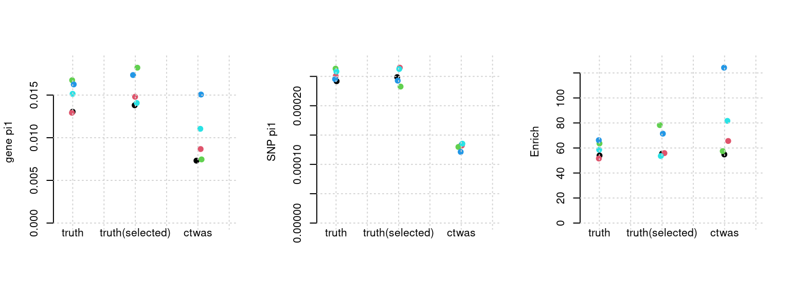

Version	Author	Date
972fe6d	simingz	2023-06-05

print("When running with L= 5 in final step:")

[1] "When running with L= 5 in final step:"

plot_PIP(1, runtag, simutags)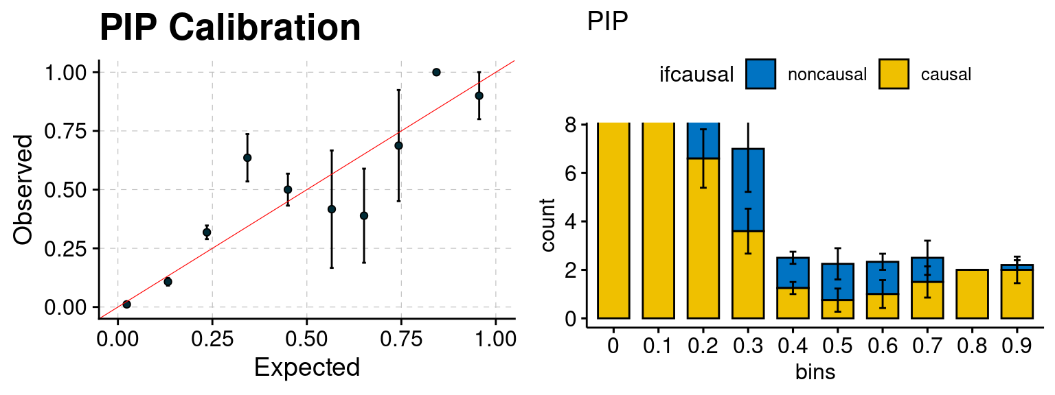

Version	Author	Date
972fe6d	simingz	2023-06-05

print("When running with L= 1 in final step:")

[1] "When running with L= 1 in final step:"

plot_PIP(2, runtag, simutags)

Version	Author	Date
3631063	simingz	2023-06-05
972fe6d	simingz	2023-06-05

# plot_fusion_coloc(configtag, runtag, simutags)
# # plot_focus(configtag, runtag, simutags)
# print("FOCUS result is null")
# plot_smr(configtag, runtag, simutags)

simutags <- paste(2, 1:5, sep = "-")
plot_par(1, runtag, simutags)

simulations  2-1 2-2 2-3 2-4 2-5 : mean gene PVE: 0.02163766 , mean SNP PVE: 0.09827806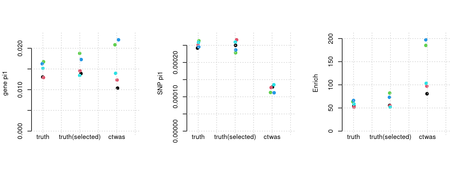

Version	Author	Date
3631063	simingz	2023-06-05
972fe6d	simingz	2023-06-05

print("When running with L= 5 in final step:")

[1] "When running with L= 5 in final step:"

plot_PIP(1, runtag, simutags)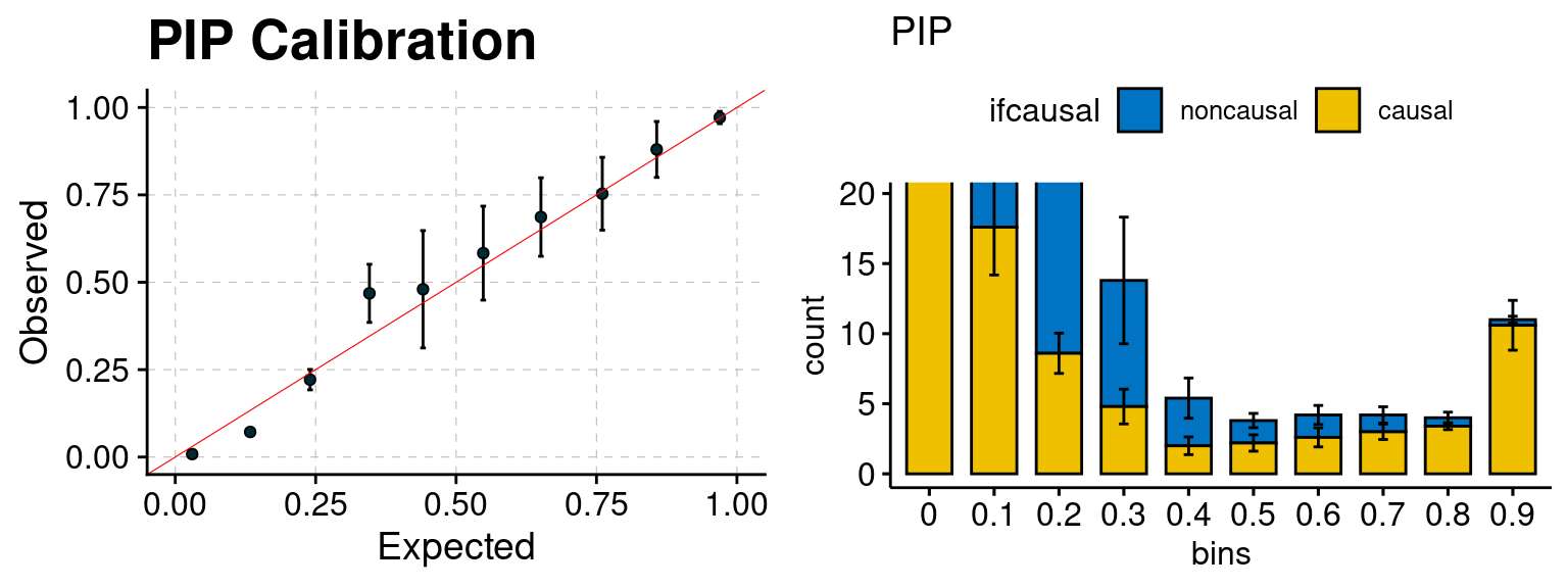

Version	Author	Date
3631063	simingz	2023-06-05
972fe6d	simingz	2023-06-05

print("When running with L= 1 in final step:")

[1] "When running with L= 1 in final step:"

plot_PIP(2, runtag, simutags)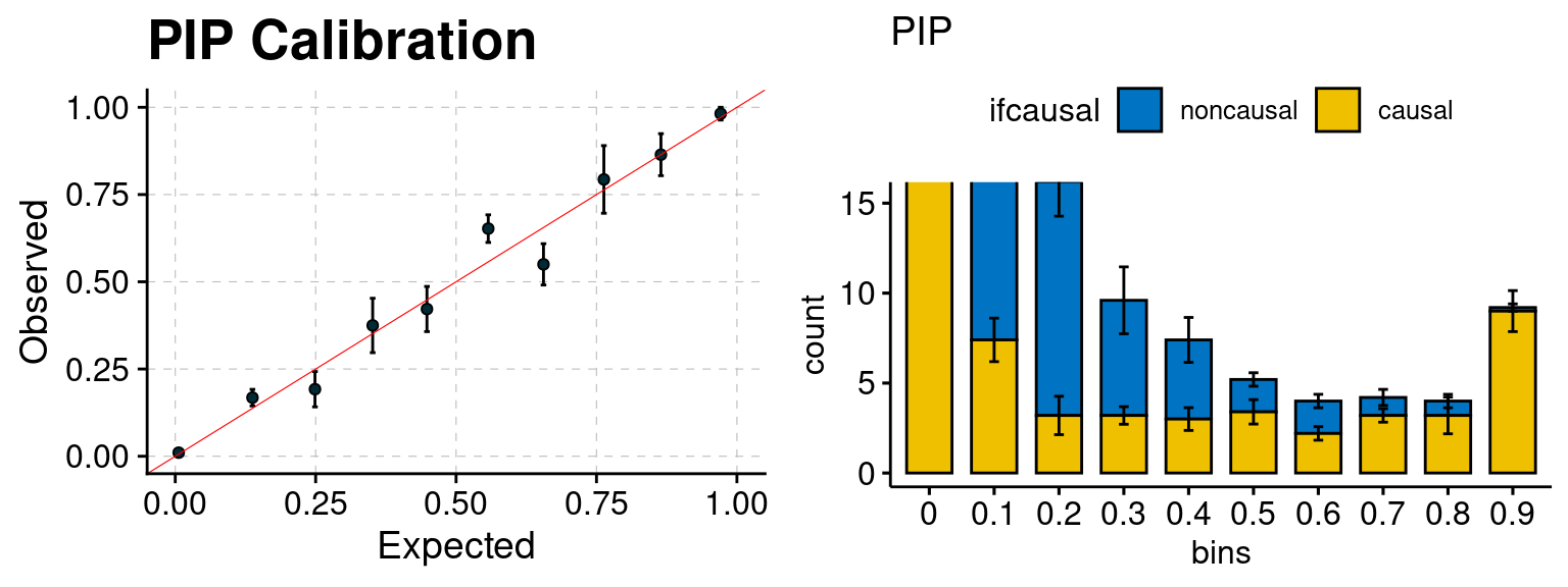

Version	Author	Date
3631063	simingz	2023-06-05
972fe6d	simingz	2023-06-05

# plot_fusion_coloc(configtag, runtag, simutags)
# #plot_focus(configtag, runtag, simutags)
# plot_smr(configtag, runtag, simutags)

simutags <- paste(3, 1:5, sep = "-")
plot_par(1, runtag, simutags)

simulations  3-1 3-2 3-3 3-4 3-5 : mean gene PVE: 0.02007495 , mean SNP PVE: 0.1991711

Version	Author	Date
3631063	simingz	2023-06-05
972fe6d	simingz	2023-06-05

print("When running with L= 5 in final step:")

[1] "When running with L= 5 in final step:"

plot_PIP(1, runtag, simutags)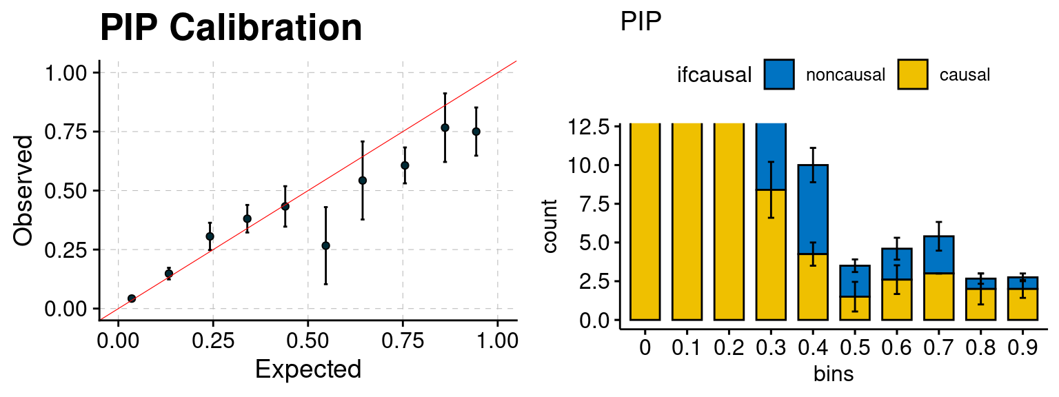

Version	Author	Date
3631063	simingz	2023-06-05
972fe6d	simingz	2023-06-05

print("When running with L= 1 in final step:")

[1] "When running with L= 1 in final step:"

plot_PIP(2, runtag, simutags)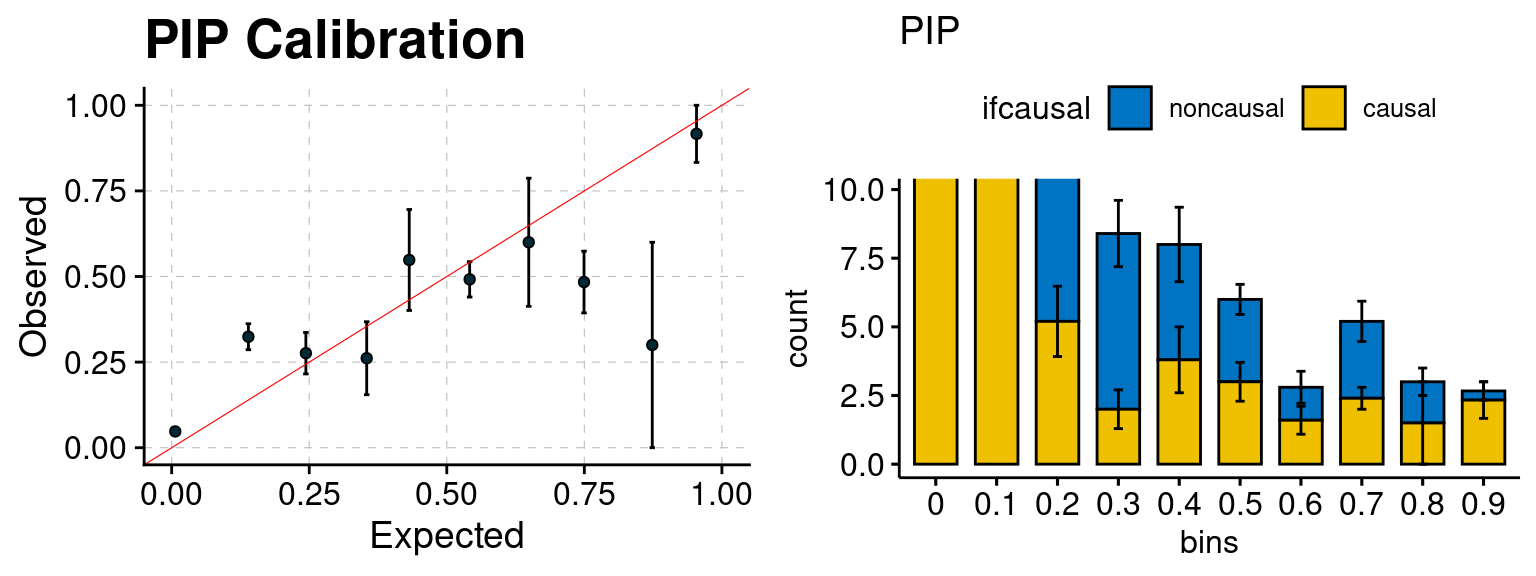

Version	Author	Date
3631063	simingz	2023-06-05
972fe6d	simingz	2023-06-05

# plot_fusion_coloc(configtag, runtag, simutags)
# #plot_focus(configtag, runtag, simutags)
# plot_smr(configtag, runtag, simutags)

simutags <- paste(4, 1:5, sep = "-")
plot_par(1, runtag, simutags)

simulations  4-1 4-2 4-3 4-4 4-5 : mean gene PVE: 0.05019153 , mean SNP PVE: 0.1992051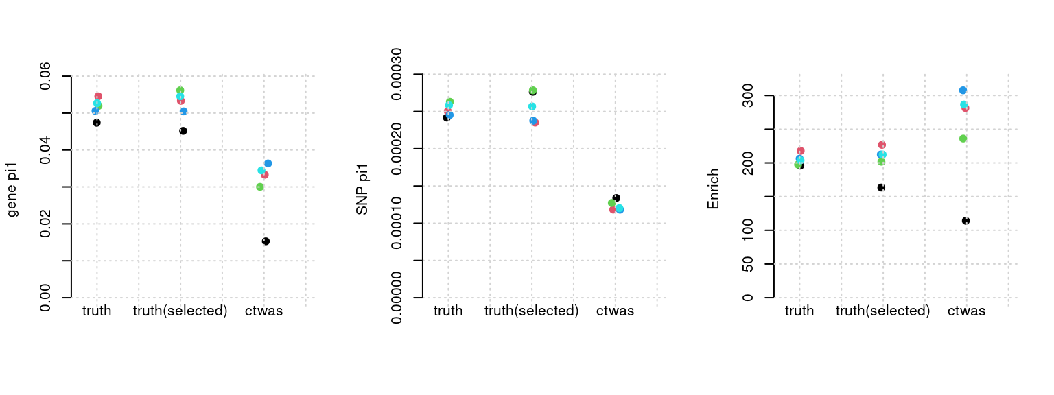

Version	Author	Date
3631063	simingz	2023-06-05
972fe6d	simingz	2023-06-05

print("When running with L= 5 in final step:")

[1] "When running with L= 5 in final step:"

plot_PIP(1, runtag, simutags)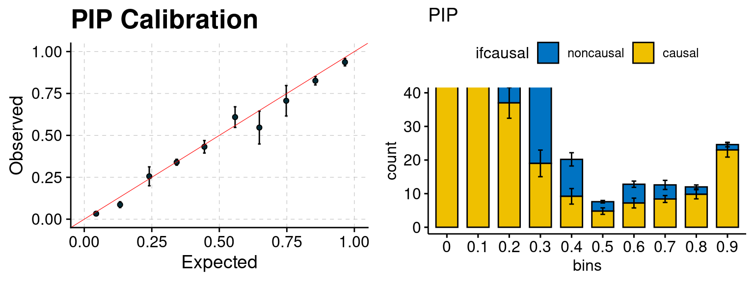

Version	Author	Date
972fe6d	simingz	2023-06-05

print("When running with L= 1 in final step:")

[1] "When running with L= 1 in final step:"

plot_PIP(2, runtag, simutags)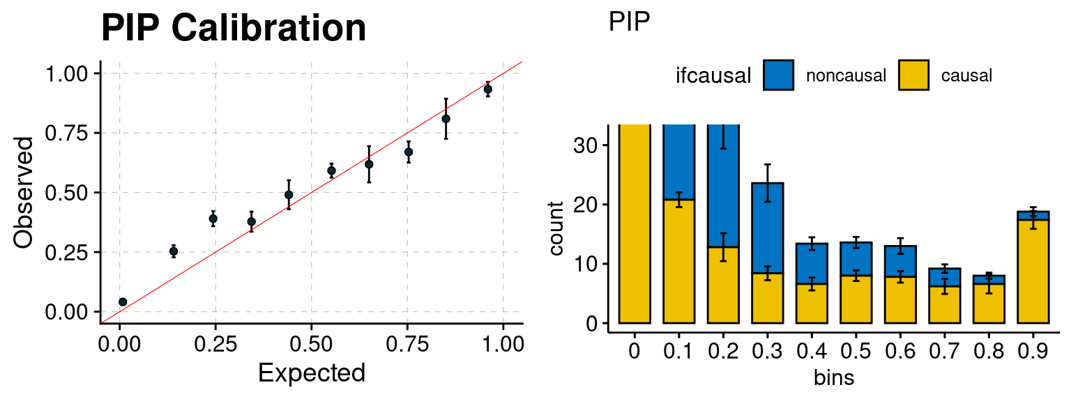

Version	Author	Date
972fe6d	simingz	2023-06-05

# plot_fusion_coloc(configtag, runtag, simutags)
# #plot_focus(configtag, runtag, simutags)
# plot_smr(configtag, runtag, simutags)

simutags <- paste(5, c(1:5), sep = "-")
plot_par(1, runtag, simutags)

simulations  5-1 5-2 5-3 5-4 5-5 : mean gene PVE: 0.100387 , mean SNP PVE: 0.1992397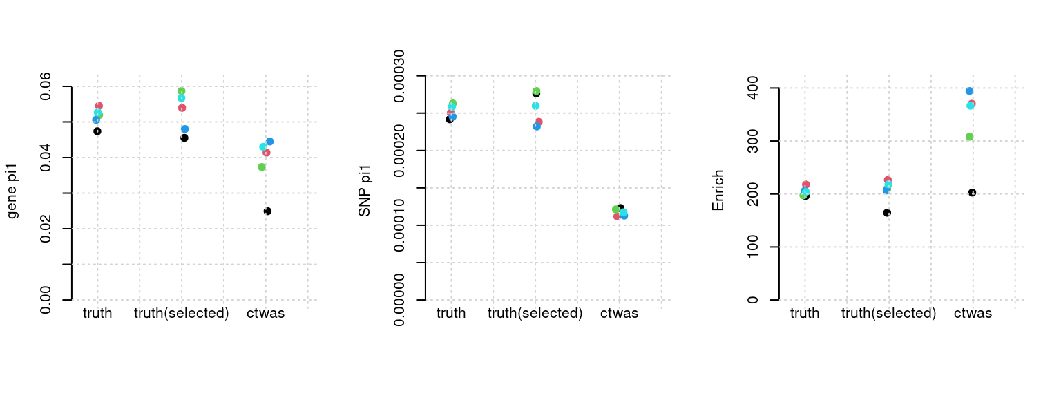

Version	Author	Date
972fe6d	simingz	2023-06-05

print("When running with L= 5 in final step:")

[1] "When running with L= 5 in final step:"

plot_PIP(1, runtag, simutags)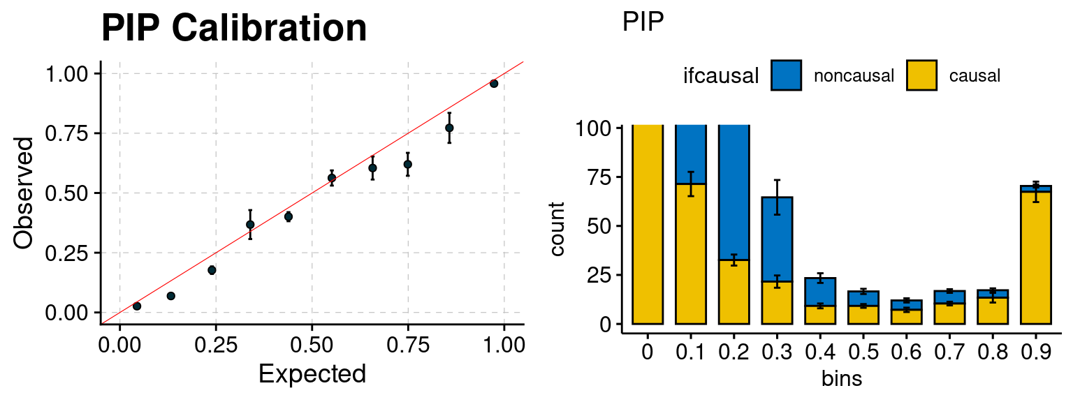

Version	Author	Date
972fe6d	simingz	2023-06-05

print("When running with L= 1 in final step:")

[1] "When running with L= 1 in final step:"

plot_PIP(2, runtag, simutags)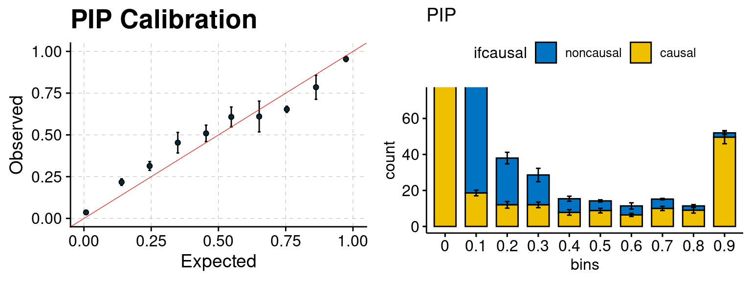

Version	Author	Date
972fe6d	simingz	2023-06-05

simutags <- paste(6, 1:20, sep = "-")
plot_par(1, runtag, simutags)

simulations  6-1 6-2 6-3 6-4 6-5 6-6 6-7 6-8 6-9 6-10 6-11 6-12 6-13 6-14 6-15 6-16 6-17 6-18 6-19 6-20 : mean gene PVE: 0.005149389 , mean SNP PVE: 0.2005157

print("When running with L= 5 in final step:")

[1] "When running with L= 5 in final step:"

plot_PIP(3, runtag, simutags)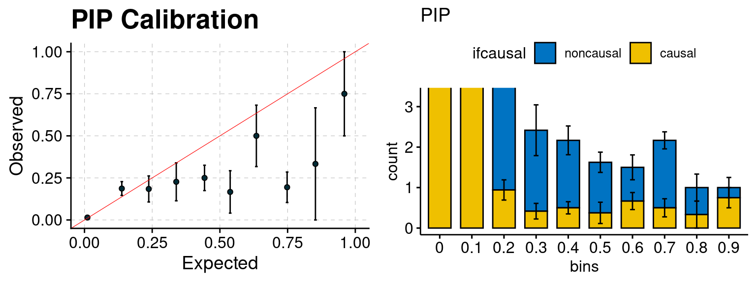

print("When running with L= 1 in final step:")

[1] "When running with L= 1 in final step:"

plot_PIP(2, runtag, simutags)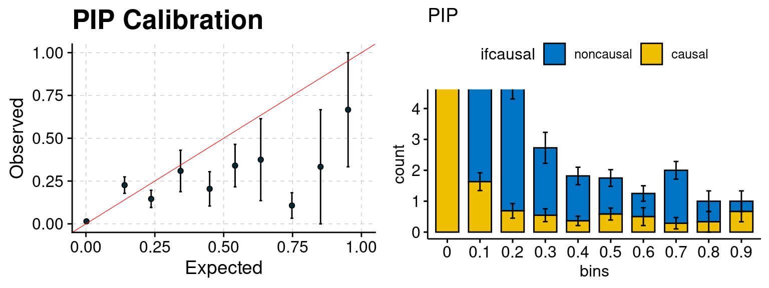

simutags <- paste(7, 1:20, sep = "-")
plot_par(1, runtag, simutags)

simulations  7-1 7-2 7-3 7-4 7-5 7-6 7-7 7-8 7-9 7-10 7-11 7-12 7-13 7-14 7-15 7-16 7-17 7-18 7-19 7-20 : mean gene PVE: 0.01029597 , mean SNP PVE: 0.2004961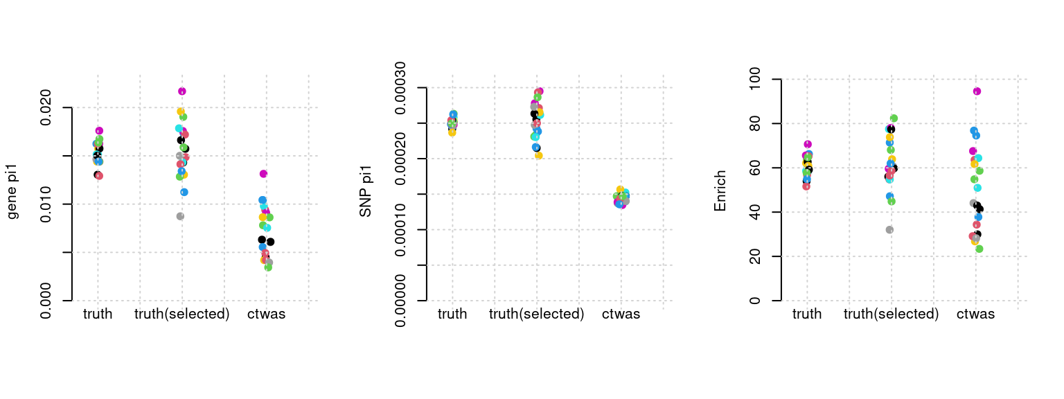

print("When running with L= 5 in final step:")

[1] "When running with L= 5 in final step:"

plot_PIP(3, runtag, simutags)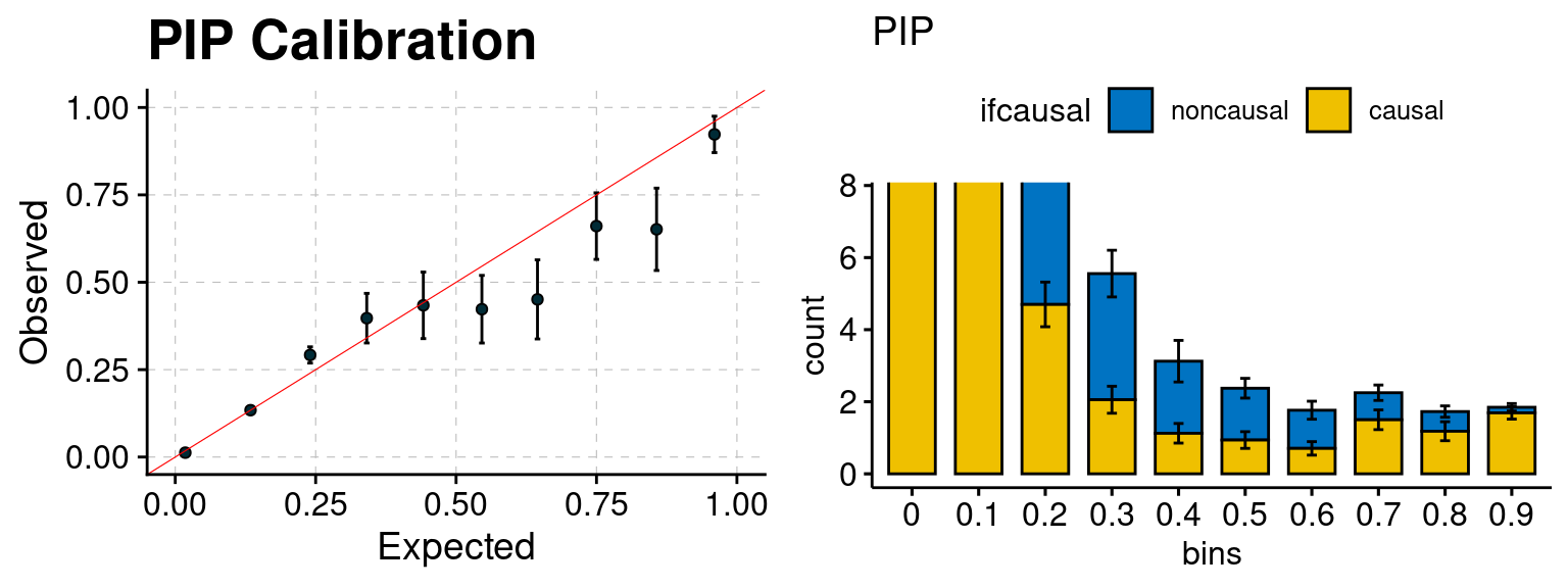

print("When running with L= 1 in final step:")

[1] "When running with L= 1 in final step:"

plot_PIP(2, runtag, simutags)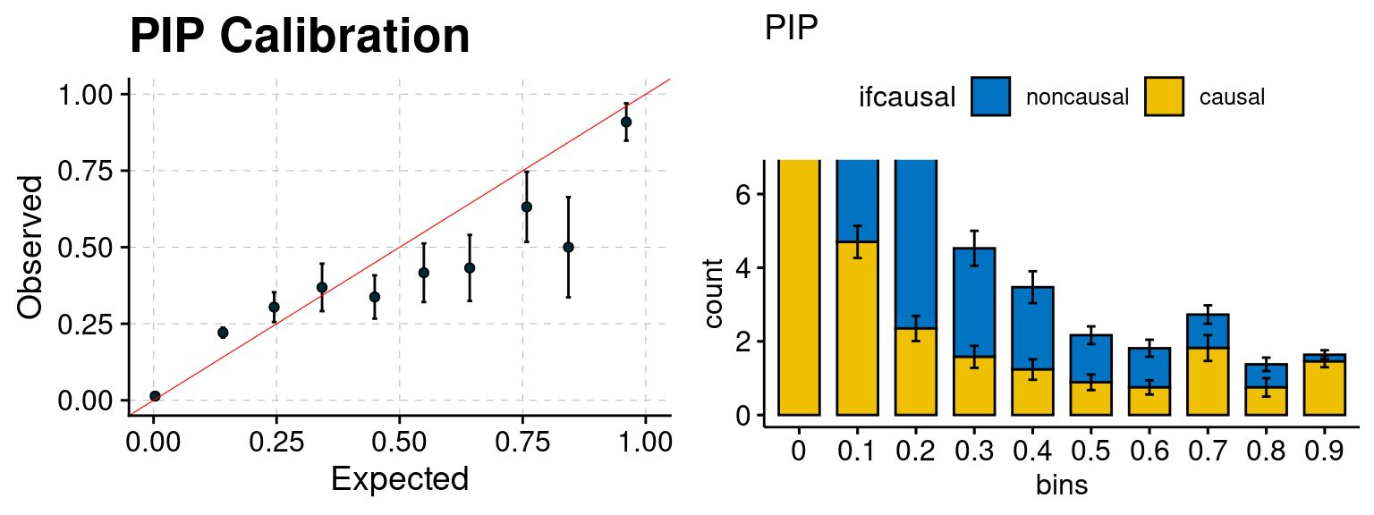

simutags <- paste(11, 1:20, sep = "-")
plot_par(1, runtag, simutags)

simulations  11-1 11-2 11-3 11-4 11-5 11-6 11-7 11-8 11-9 11-10 11-11 11-12 11-13 11-14 11-15 11-16 11-17 11-18 11-19 11-20 : mean gene PVE: 0.02058041 , mean SNP PVE: 0.2004526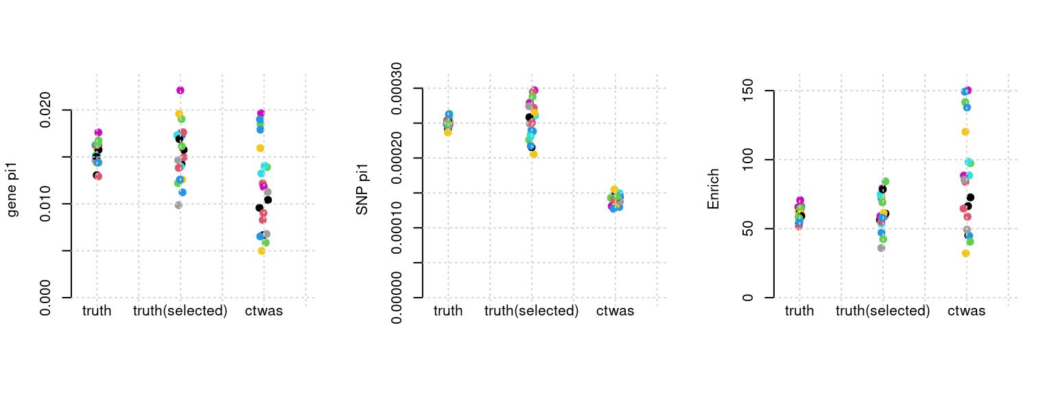

print("When running with L= 5 in final step:")

[1] "When running with L= 5 in final step:"

plot_PIP(3, runtag, simutags)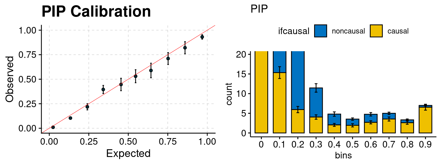

print("When running with L= 1 in final step:")

[1] "When running with L= 1 in final step:"

plot_PIP(2, runtag, simutags)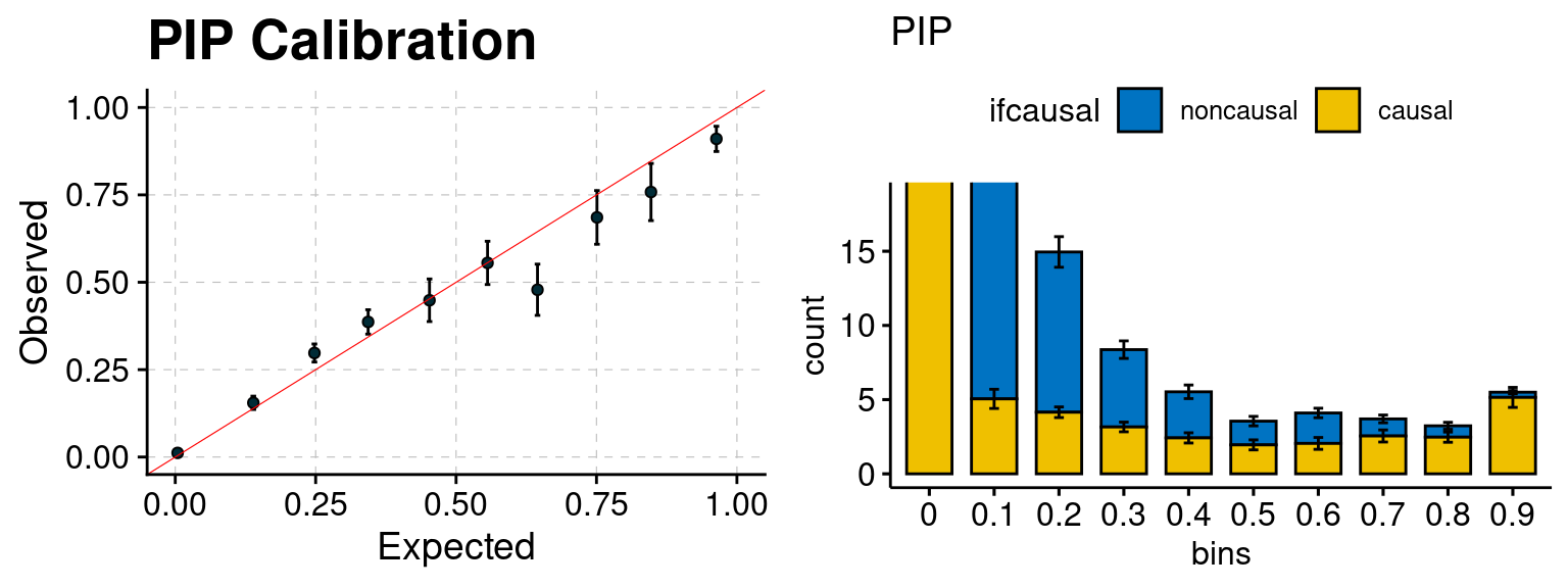

simutags <- paste(8, c(1:13,15:20), sep = "-")
plot_par(1, runtag, simutags)

simulations  8-1 8-2 8-3 8-4 8-5 8-6 8-7 8-8 8-9 8-10 8-11 8-12 8-13 8-15 8-16 8-17 8-18 8-19 8-20 : mean gene PVE: 0.05025694 , mean SNP PVE: 0.2004765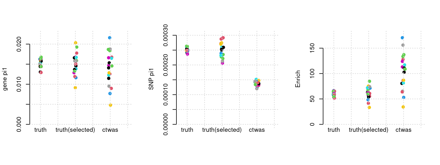

print("When running with L= 5 in final step:")

[1] "When running with L= 5 in final step:"

plot_PIP(3, runtag, simutags)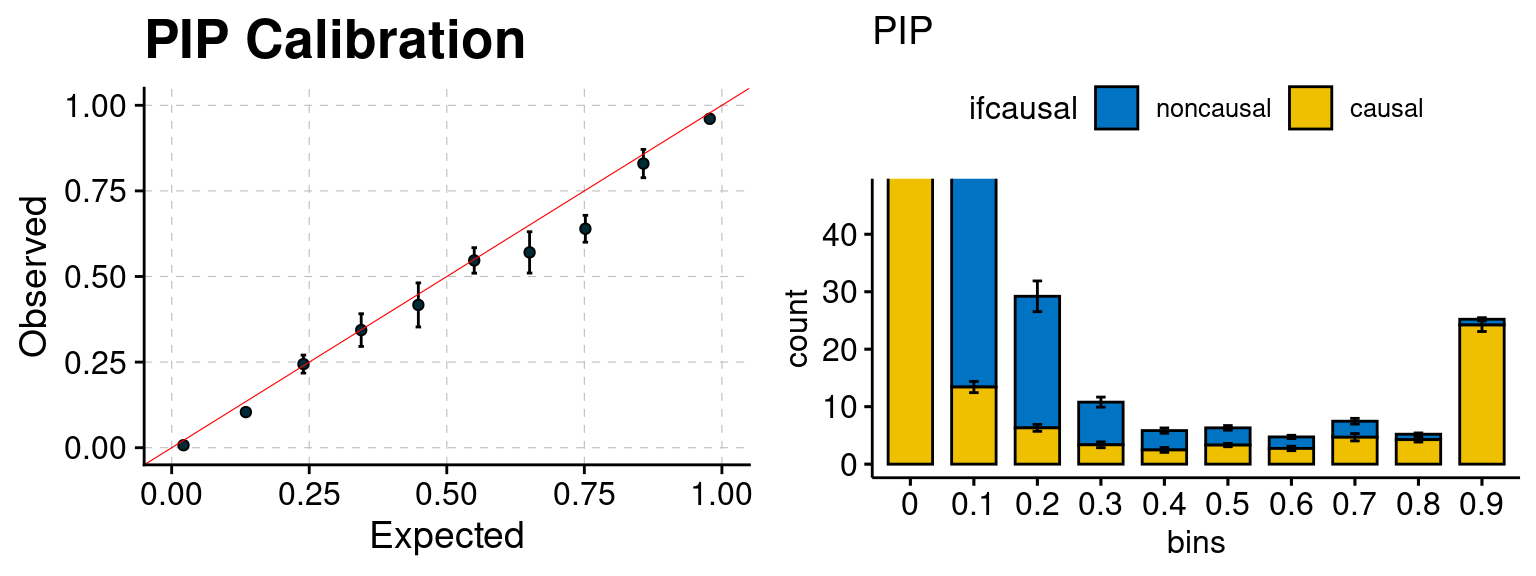

print("When running with L= 1 in final step:")

[1] "When running with L= 1 in final step:"

plot_PIP(2, runtag, simutags)

simutags <- paste(9, 1:20, sep = "-")
plot_par(1, runtag, simutags)

simulations  9-1 9-2 9-3 9-4 9-5 9-6 9-7 9-8 9-9 9-10 9-11 9-12 9-13 9-14 9-15 9-16 9-17 9-18 9-19 9-20 : mean gene PVE: 0.1024528 , mean SNP PVE: 0.2001043

print("When running with L= 5 in final step:")

[1] "When running with L= 5 in final step:"

plot_PIP(3, runtag, simutags)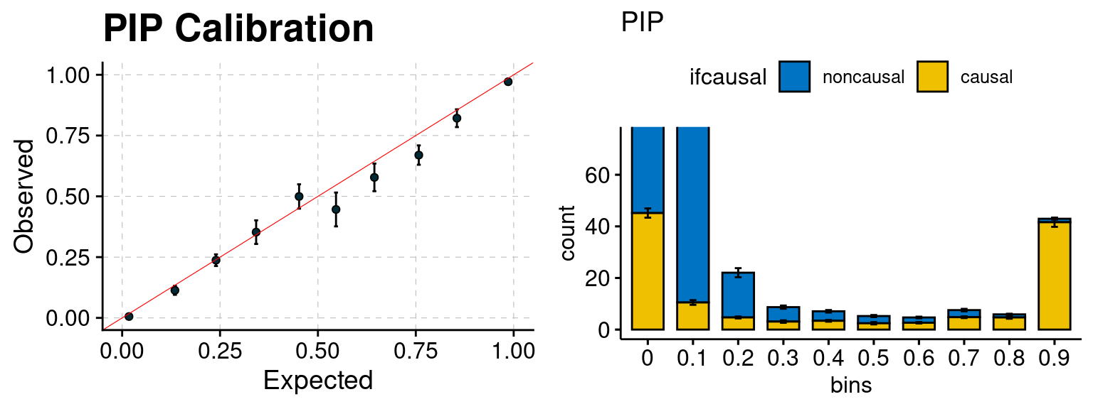

print("When running with L= 1 in final step:")

[1] "When running with L= 1 in final step:"

plot_PIP(2, runtag, simutags)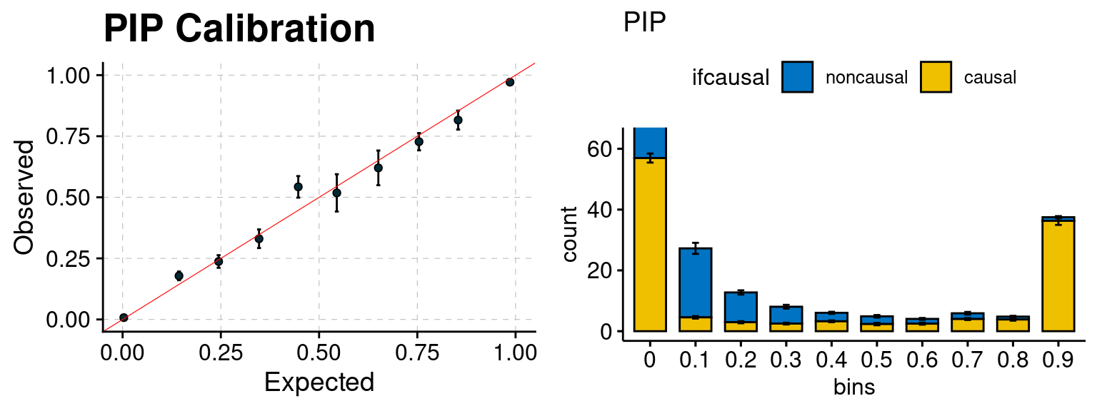

sessionInfo()

R version 4.1.0 (2021-05-18)
Platform: x86_64-pc-linux-gnu (64-bit)
Running under: CentOS Linux 7 (Core)

Matrix products: default
BLAS:   /software/R-4.1.0-no-openblas-el7-x86_64/lib64/R/lib/libRblas.so
LAPACK: /software/R-4.1.0-no-openblas-el7-x86_64/lib64/R/lib/libRlapack.so

locale:
 [1] LC_CTYPE=en_US.UTF-8 LC_NUMERIC=C         LC_TIME=C           
 [4] LC_COLLATE=C         LC_MONETARY=C        LC_MESSAGES=C       
 [7] LC_PAPER=C           LC_NAME=C            LC_ADDRESS=C        
[10] LC_TELEPHONE=C       LC_MEASUREMENT=C     LC_IDENTIFICATION=C 

attached base packages:
[1] stats     graphics  grDevices utils     datasets  methods   base     

other attached packages:
 [1] ggpubr_0.4.0      plotrix_3.8-2     cowplot_1.1.1     stringr_1.4.0    
 [5] plyr_1.8.6        tidyr_1.1.3       plotly_4.9.4.1    ggplot2_3.3.5    
 [9] data.table_1.14.0 ctwas_0.1.35     

loaded via a namespace (and not attached):
 [1] httr_1.4.2        sass_0.4.0        jsonlite_1.7.2    viridisLite_0.4.0
 [5] foreach_1.5.1     carData_3.0-4     pgenlibr_0.3.2    logging_0.10-108 
 [9] bslib_0.4.2       assertthat_0.2.1  highr_0.9         cellranger_1.1.0 
[13] yaml_2.2.1        pillar_1.6.1      backports_1.2.1   lattice_0.20-44  
[17] glue_1.4.2        digest_0.6.27     promises_1.2.0.1  ggsignif_0.6.2   
[21] colorspace_2.0-2  htmltools_0.5.5   httpuv_1.6.1      Matrix_1.3-3     
[25] pkgconfig_2.0.3   broom_0.7.8       haven_2.4.1       purrr_0.3.4      
[29] scales_1.1.1      whisker_0.4       openxlsx_4.2.4    later_1.2.0      
[33] rio_0.5.27        git2r_0.28.0      tibble_3.1.2      farver_2.1.0     
[37] generics_0.1.0    car_3.0-11        ellipsis_0.3.2    cachem_1.0.5     
[41] withr_2.5.0       lazyeval_0.2.2    cli_3.6.1         readxl_1.3.1     
[45] magrittr_2.0.1    crayon_1.5.2      evaluate_0.20     fs_1.6.1         
[49] fansi_0.5.0       rstatix_0.7.0     forcats_0.5.1     foreign_0.8-81   
[53] tools_4.1.0       hms_1.1.0         lifecycle_1.0.3   munsell_0.5.0    
[57] ggsci_2.9         zip_2.2.0         compiler_4.1.0    jquerylib_0.1.4  
[61] rlang_1.1.0       grid_4.1.0        iterators_1.0.13  rstudioapi_0.13  
[65] htmlwidgets_1.5.3 labeling_0.4.2    rmarkdown_2.21    gtable_0.3.0     
[69] codetools_0.2-18  abind_1.4-5       DBI_1.1.1         curl_4.3.2       
[73] R6_2.5.0          gridExtra_2.3     knitr_1.42        dplyr_1.0.7      
[77] fastmap_1.1.0     utf8_1.2.1        workflowr_1.6.2   rprojroot_2.0.2  
[81] stringi_1.6.2     Rcpp_1.0.9        vctrs_0.3.8       tidyselect_1.1.1 
[85] xfun_0.38

Simulations to test ctwas summary stats version, 45k samples, a few new setings required

Analysis description

Data

Analysis

ctwas

ctwas results

`ctwas` results