Gaussian mean estimation in simulated data sets
Zhengrong Xing, Peter Carbonetto and Matthew Stephens
Last updated: 2020-06-16
Checks: 7 0
Knit directory: smash-paper/analysis/
This reproducible R Markdown analysis was created with workflowr (version 1.6.2). The Checks tab describes the reproducibility checks that were applied when the results were created. The Past versions tab lists the development history.
Great! Since the R Markdown file has been committed to the Git repository, you know the exact version of the code that produced these results.
Great job! The global environment was empty. Objects defined in the global environment can affect the analysis in your R Markdown file in unknown ways. For reproduciblity it’s best to always run the code in an empty environment.
The command set.seed(1) was run prior to running the code in the R Markdown file. Setting a seed ensures that any results that rely on randomness, e.g. subsampling or permutations, are reproducible.
Great job! Recording the operating system, R version, and package versions is critical for reproducibility.
Nice! There were no cached chunks for this analysis, so you can be confident that you successfully produced the results during this run.
Great job! Using relative paths to the files within your workflowr project makes it easier to run your code on other machines.
Great! You are using Git for version control. Tracking code development and connecting the code version to the results is critical for reproducibility.
The results in this page were generated with repository version ec646cc. See the Past versions tab to see a history of the changes made to the R Markdown and HTML files.
Note that you need to be careful to ensure that all relevant files for the analysis have been committed to Git prior to generating the results (you can use wflow_publish or wflow_git_commit). workflowr only checks the R Markdown file, but you know if there are other scripts or data files that it depends on. Below is the status of the Git repository when the results were generated:
Ignored files:
    Ignored:    dsc/code/Wavelab850/MEXSource/CPAnalysis.mexmac
    Ignored:    dsc/code/Wavelab850/MEXSource/DownDyadHi.mexmac
    Ignored:    dsc/code/Wavelab850/MEXSource/DownDyadLo.mexmac
    Ignored:    dsc/code/Wavelab850/MEXSource/FAIPT.mexmac
    Ignored:    dsc/code/Wavelab850/MEXSource/FCPSynthesis.mexmac
    Ignored:    dsc/code/Wavelab850/MEXSource/FMIPT.mexmac
    Ignored:    dsc/code/Wavelab850/MEXSource/FWPSynthesis.mexmac
    Ignored:    dsc/code/Wavelab850/MEXSource/FWT2_PO.mexmac
    Ignored:    dsc/code/Wavelab850/MEXSource/FWT_PBS.mexmac
    Ignored:    dsc/code/Wavelab850/MEXSource/FWT_PO.mexmac
    Ignored:    dsc/code/Wavelab850/MEXSource/FWT_TI.mexmac
    Ignored:    dsc/code/Wavelab850/MEXSource/IAIPT.mexmac
    Ignored:    dsc/code/Wavelab850/MEXSource/IMIPT.mexmac
    Ignored:    dsc/code/Wavelab850/MEXSource/IWT2_PO.mexmac
    Ignored:    dsc/code/Wavelab850/MEXSource/IWT_PBS.mexmac
    Ignored:    dsc/code/Wavelab850/MEXSource/IWT_PO.mexmac
    Ignored:    dsc/code/Wavelab850/MEXSource/IWT_TI.mexmac
    Ignored:    dsc/code/Wavelab850/MEXSource/LMIRefineSeq.mexmac
    Ignored:    dsc/code/Wavelab850/MEXSource/MedRefineSeq.mexmac
    Ignored:    dsc/code/Wavelab850/MEXSource/UpDyadHi.mexmac
    Ignored:    dsc/code/Wavelab850/MEXSource/UpDyadLo.mexmac
    Ignored:    dsc/code/Wavelab850/MEXSource/WPAnalysis.mexmac
    Ignored:    dsc/code/Wavelab850/MEXSource/dct_ii.mexmac
    Ignored:    dsc/code/Wavelab850/MEXSource/dct_iii.mexmac
    Ignored:    dsc/code/Wavelab850/MEXSource/dct_iv.mexmac
    Ignored:    dsc/code/Wavelab850/MEXSource/dst_ii.mexmac
    Ignored:    dsc/code/Wavelab850/MEXSource/dst_iii.mexmac
Note that any generated files, e.g. HTML, png, CSS, etc., are not included in this status report because it is ok for generated content to have uncommitted changes.
These are the previous versions of the repository in which changes were made to the R Markdown (analysis/gaussmeanest.Rmd) and HTML (docs/gaussmeanest.html) files. If you’ve configured a remote Git repository (see ?wflow_git_remote), click on the hyperlinks in the table below to view the files as they were in that past version.
| File | Version | Author | Date | Message |
|---|---|---|---|---|
| Rmd | ec646cc | Peter Carbonetto | 2020-06-16 | wflow_publish(“gaussmeanest.Rmd”) |
| html | 66b45bb | Peter Carbonetto | 2020-06-16 | Added simulated data set to Corner signal plot in “gaussmeanest” |
| Rmd | 571a221 | Peter Carbonetto | 2020-06-16 | wflow_publish(“gaussmeanest.Rmd”) |
| html | bc790ae | Peter Carbonetto | 2020-06-16 | Added example simulated data set to “Spikes” signal plot in |
| Rmd | 935bef6 | Peter Carbonetto | 2020-06-16 | wflow_publish(“gaussmeanest.Rmd”) |
| Rmd | b87fe83 | Peter Carbonetto | 2020-01-02 | Working on code to illustrate methods applied to Spikes data. |
| html | 19c136d | Peter Carbonetto | 2019-12-31 | Small adjustment to the code in gaussmeanest analysis. |
| Rmd | 992ee9c | Peter Carbonetto | 2019-12-31 | wflow_publish(“gaussmeanest.Rmd”) |
| html | 436e150 | Peter Carbonetto | 2019-12-31 | Added bar plots to gaussmeanest analysis summarizing results from all |
| Rmd | 703f5a2 | Peter Carbonetto | 2019-12-31 | wflow_publish(“gaussmeanest.Rmd”) |
| html | f780a43 | Peter Carbonetto | 2019-12-20 | Adjusted the bar chart settings. |
| Rmd | 70dedc0 | Peter Carbonetto | 2019-12-20 | wflow_publish(“gaussmeanest.Rmd”) |
| html | 3cdef11 | Peter Carbonetto | 2019-12-20 | Added bar charts to gaussmeanest analysis summarizing results of |
| Rmd | 02f9167 | Peter Carbonetto | 2019-12-20 | wflow_publish(“gaussmeanest.Rmd”) |
| html | c8548d5 | Peter Carbonetto | 2019-12-20 | Re-built gaussmeanest analysis after making some of the plotting code |
| Rmd | 4d7aae3 | Peter Carbonetto | 2019-12-20 | wflow_publish(“gaussmeanest.Rmd”) |
| html | 8998bb8 | Peter Carbonetto | 2019-12-20 | Re-built gaussmeanest analysis after Zhengrong’s recent additions. |
| Rmd | 85aa594 | Peter Carbonetto | 2019-12-20 | wflow_publish(“gaussmeanest.Rmd”) |
| Rmd | f0221c5 | Zhengrong Xing | 2019-10-27 | address some reviewer comments |
| html | f0221c5 | Zhengrong Xing | 2019-10-27 | address some reviewer comments |
| html | 74aff51 | Peter Carbonetto | 2018-12-20 | Re-built gauss_shiny_setup and gaussmeanest pages. |
| Rmd | 86da808 | Peter Carbonetto | 2018-12-10 | Added pointers to dsc/README in relevant R Markdown files. |
| html | 8caff70 | Peter Carbonetto | 2018-12-06 | Re-built the workflowr pages after several minor changes to the text |
| Rmd | c589dbb | Peter Carbonetto | 2018-12-06 | wflow_publish(c(“index.Rmd”, “gaussian_signals.Rmd”, |
| html | ee71f27 | Peter Carbonetto | 2018-12-04 | Made a few small adjustments to the text in the “gaussianmeanest” analysis. |
| Rmd | eb6cc34 | Peter Carbonetto | 2018-12-04 | wflow_publish(“gaussmeanest.Rmd”) |
| html | 05684ba | Peter Carbonetto | 2018-12-04 | Ran wflow_publish(“gaussmeanest.Rmd”) to populate the webpage. |
| Rmd | 9a67b48 | Peter Carbonetto | 2018-12-02 | Moved dsc results file. |
| Rmd | 049dcbb | Peter Carbonetto | 2018-11-08 | Moved around some files and revised TOC in home page. |
In this analysis, we assess the ability of different signal denoising methods to recover the true signal after being provided with Gaussian-distributed observations of the signal. We consider scenarios in which the data have homoskedastic errors (constant variance) and heteroskedastic errors (non-constant variance).
Since the simulation experiments are computationally intensive, here we only illustrate the application of the signal denoising methods, and create plots summarizing the results of the full experiments; the full experiments were implemented separately. (For instructions on re-running these simulation experiments, see the README in the “dsc” directory of the git repository).
Set up environment
Load the ggplot2 and cowplot packages, and the functions definining the mean and variances used to simulate the data.
library(plyr)
library(smashr)
library(ggplot2)
library(cowplot)
source("../code/signals.R")
source("../code/gaussmeanest.functions.R")
theme_set(theme_cowplot())
Load results
Load the results of the simulation experiments.
load("../output/dscr.RData")Simulated data with constant variances
This plot reproduces Fig. 2 of the manuscript, which compares the accuracy of the mean curves estimated from the data sets that were simulated using the “Spikes” mean function with constant variance and a signal-to-noise ratio of 3.
First, extract the results used to generate this plot, and transform them into a data frame suitable for plotting using ggplot2.
pdat <- get.results.homosked(res,"sp.3.v1")Create the combined boxplot and violin plot using ggplot2.
pdat <-
  transform(pdat,
            method = factor(method,
                            names(sort(tapply(pdat$mise,pdat$method,mean),
                                       decreasing = TRUE))))
p <- ggplot(pdat,aes(x = method,y = mise,fill = method.type)) +
     geom_violin(fill = "skyblue",color = "skyblue") +
     geom_boxplot(width = 0.15,outlier.shape = NA) +
     scale_y_continuous(breaks = seq(6,16,2)) +
     scale_fill_manual(values = c("darkorange","dodgerblue","gold"),
                       guide = FALSE) +
     coord_flip() +
     labs(x = "",y = "MISE") +
     theme(axis.line = element_blank(),
           axis.ticks.y = element_blank())
print(p)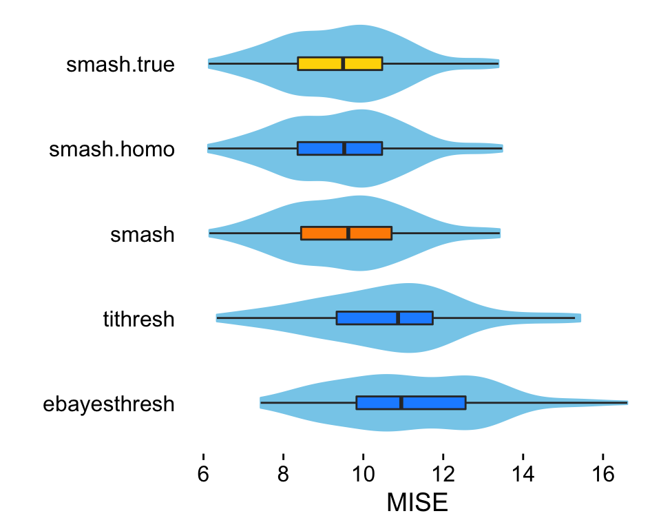
From this plot, we see that the three variants of SMASH all outperformed EbayesThresh and TI thresholding in this setting.
These plots summarize the results for all 7 simulation scenarios and the two signal-to-noise ratios (1 and 3), including the “Spikes” scenario shown in greater detail in the violin plot above.
create.bar.plots.homosked(rbind(
  data.frame(sim = "sp",  snr = 1,get.results.homosked(res,"sp.1.v1")),
  data.frame(sim = "bump",snr = 1,get.results.homosked(res,"bump.1.v1")),
  data.frame(sim = "blkp",snr = 1,get.results.homosked(res,"blk.1.v1")),
  data.frame(sim = "ang", snr = 1,get.results.homosked(res,"ang.1.v1")),
  data.frame(sim = "dop", snr = 1,get.results.homosked(res,"dop.1.v1")),
  data.frame(sim = "blip",snr = 1,get.results.homosked(res,"blip.1.v1")),
  data.frame(sim = "cor", snr = 1,get.results.homosked(res,"cor.1.v1")),
  data.frame(sim = "sp",  snr = 3,get.results.homosked(res,"sp.3.v1")),
  data.frame(sim = "bump",snr = 3,get.results.homosked(res,"bump.3.v1")),
  data.frame(sim = "blkp",snr = 3,get.results.homosked(res,"blk.3.v1")),
  data.frame(sim = "ang", snr = 3,get.results.homosked(res,"ang.3.v1")),
  data.frame(sim = "dop", snr = 3,get.results.homosked(res,"dop.3.v1")),
  data.frame(sim = "blip",snr = 3,get.results.homosked(res,"blip.3.v1")),
  data.frame(sim = "cor", snr = 3,get.results.homosked(res,"cor.3.v1"))))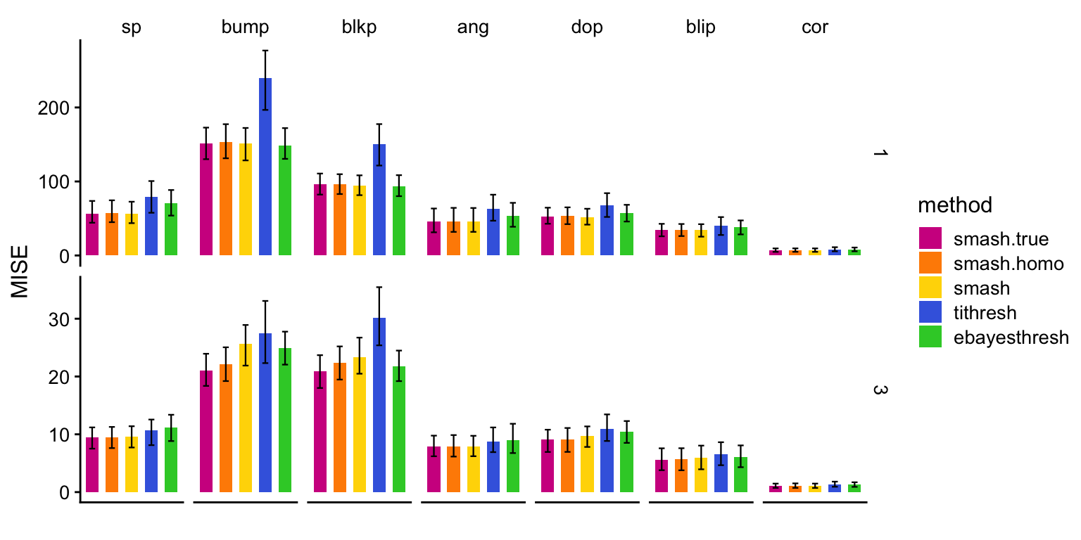
Next, we compare the same methods in simulated data sets with heteroskedastic errors.
Simulated data with heteroskedastic errors: “Spikes” mean signal and “Clipped Blocks” variance
In this scenario, the data sets were simulated using the “Spikes” mean function and the “Clipped Blocks” variance function. The next two plots reproduce part of Fig. 3 in the manuscript.
This plot shows the mean function as an orange line, the +/- 2 standard deviations as dashed, light blue lines, and an example simulated data set (black circles):
t         <- (1:1024)/1024
mu        <- spike.fn(t,"mean")
sigma.ini <- sqrt(cblocks.fn(t,"var"))
sd.fn     <- sigma.ini/mean(sigma.ini) * sd(mu)/3
x.sim     <- rnorm(1024,mu,sd.fn)
par(cex.axis = 1,cex.lab = 1.25)
plot(mu,type = "l", ylim = c(-0.05,1),col = "darkorange",
     xlab = "position",ylab = "",lwd = 1.75,xaxp = c(0,1024,4),
     yaxp = c(0,1,4))
lines(mu + 2*sd.fn,col = "dodgerblue",lty = "dashed",lwd = 1.75)
lines(mu - 2*sd.fn,col = "dodgerblue",lty = "dashed",lwd = 1.75)
points(x.sim,cex = 0.7,pch = 1,col = "black")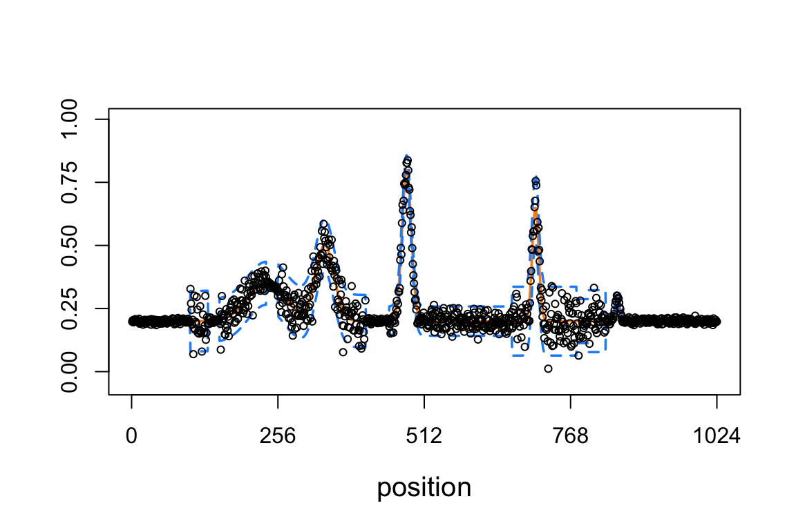
| Version | Author | Date |
|---|---|---|
| bc790ae | Peter Carbonetto | 2020-06-16 |
Next, we plot the ground-truth signal (the mean function, drawn as a black line), and the signals recovered by TI thresholding (light blue line) and SMASH (the red line) for the example simulated data set.
mu.smash <- smash(x.sim,family = "DaubLeAsymm",filter.number = 8)
mu.ti    <- ti.thresh(x.sim,method = "rmad",family = "DaubLeAsymm",
                      filter.number = 8)
par(cex.axis = 1)
plot(mu,type = "l",col = "black",lwd = 3,xlab = "position",ylab = "",
     ylim = c(-0.05,1),xaxp = c(0,1024,4),yaxp = c(0,1,4))
lines(mu.ti,col = "dodgerblue",lwd = 3)
lines(mu.smash,col = "orangered",lwd = 3)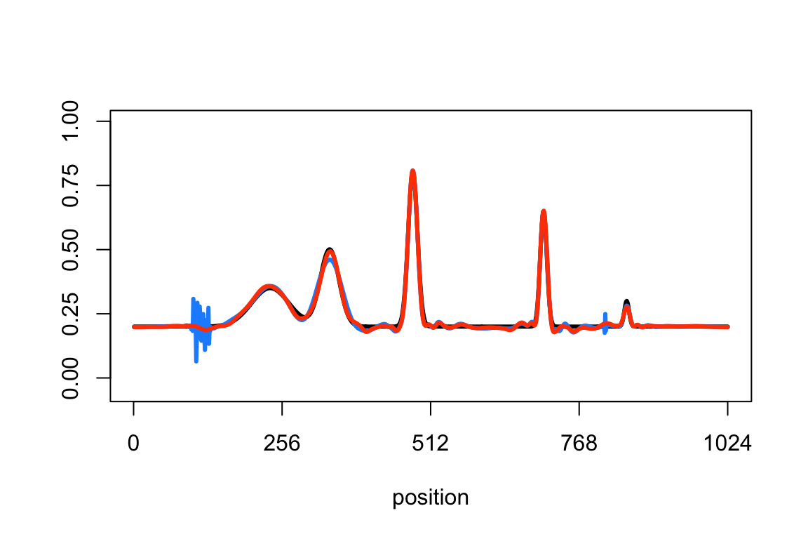
Extract the results from running the simulations.
hetero.data.smash <-
  res[res$.id == "sp.3.v5" & res$method == "smash.s8",]
hetero.data.smash.homo <-
  res[res$.id == "sp.3.v5" & res$method == "smash.homo.s8",]
hetero.data.tithresh.homo <-
  res[res$.id == "sp.3.v5" & res$method == "tithresh.homo.s8",]
hetero.data.tithresh.rmad <-
  res[res$.id == "sp.3.v5" & res$method == "tithresh.rmad.s8",]
hetero.data.tithresh.smash <-
  res[res$.id == "sp.3.v5" & res$method == "tithresh.smash.s8",]
hetero.data.tithresh.true <-
  res[res$.id == "sp.3.v5" & res$method == "tithresh.true.s8",]
hetero.data.ebayes <-
  res[res$.id == "sp.3.v5" & res$method == "ebayesthresh",]
hetero.data.smash.true <-
  res[res$.id == "sp.3.v5" & res$method == "smash.true.s8",]
Transform these results into a data frame suitable for ggplot2.
pdat <-
  rbind(data.frame(method      = "smash",
                   method.type = "est",
                   mise        = hetero.data.smash$mise),
        data.frame(method      = "smash.homo",
                   method.type = "homo",
                   mise        = hetero.data.smash.homo$mise),
        data.frame(method      = "tithresh.rmad",
                   method.type = "tithresh",
                   mise        = hetero.data.tithresh.rmad$mise),
        data.frame(method      = "tithresh.smash",
                   method.type = "tithresh",
                   mise        = hetero.data.tithresh.smash$mise),
        data.frame(method      = "tithresh.true",
                   method.type = "tithresh",
                   mise        = hetero.data.tithresh.true$mise),
        data.frame(method      = "ebayesthresh",
                   method.type = "homo",
                   mise        = hetero.data.ebayes$mise),
        data.frame(method      = "smash.true",
                   method.type = "true",
                   mise        = hetero.data.smash.true$mise))
pdat <-
  transform(pdat,
            method = factor(method,
                            names(sort(tapply(pdat$mise,pdat$method,mean),
                                       decreasing = TRUE))))
Create the combined boxplot and violin plot using ggplot2.
p <- ggplot(pdat,aes(x = method,y = mise,fill = method.type)) +
     geom_violin(fill = "skyblue",color = "skyblue") +
     geom_boxplot(width = 0.15,outlier.shape = NA) +
     scale_fill_manual(values=c("darkorange","dodgerblue","limegreen","gold"),
                       guide = FALSE) +
     coord_flip() +
     scale_y_continuous(breaks = seq(10,70,10)) +
     labs(x = "",y = "MISE") +
     theme(axis.line = element_blank(),
           axis.ticks.y = element_blank())
print(p)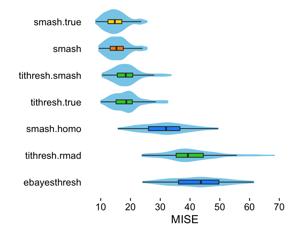
In this scenario, we see that SMASH, when allowing for heteroskedastic errors, outperforms EbayesThresh and all variants of TI thresholding (including TI thresholding when provided with the true variance). Further, SMASH performs almost as well when estimating the variance compared to when provided with the true variance.
Simulated data with heteroskedastic errors: “Corner” mean signal and “Doppler” variance
In this next scenario, the data sets were simulated using the “Corner” mean function and the “Doppler” variance function. These plots were also used in Figure 3 of the manuscript.
This plot shows the mean function as an orange line, the +/- 2 standard deviations as dashed, light blue lines, and an example simulated data set (black circles):
t         <- (1:1024)/1024
mu        <- cor.fn(t,"mean")
sigma.ini <- sqrt(doppler.fn(t,"var"))
sd.fn     <- sigma.ini/mean(sigma.ini) * sd(mu)/3
x.sim     <- rnorm(1024,mu,sd.fn)
plot(mu,type = "l",col = "darkorange",ylim = c(-0.05,1),
     xlab = "position",ylab = "",lwd = 1.75,xaxp = c(0,1024,4),
     yaxp = c(0,1,4))
lines(mu + 2*sd.fn,col = "dodgerblue",lty = "dashed",lwd = 1.75)
lines(mu - 2*sd.fn,col = "dodgerblue",lty = "dashed",lwd = 1.75)
points(x.sim,cex = 0.7,pch = 1,col = "black")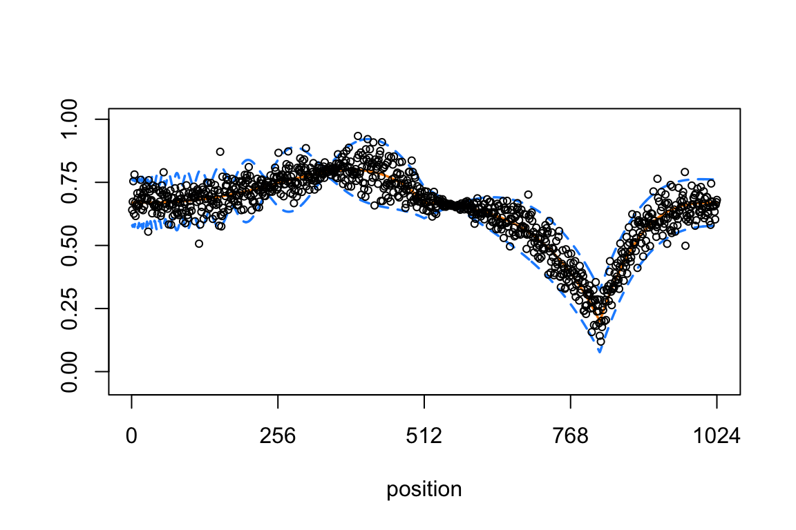
Now, we plot the ground-truth signal (the mean function, drawn as a black line) and the signals recovered by TI thresholding (light blue line) and SMASH (the red line) for one simulated dataset as an illustration
mu.smash <- smash(x.sim,family = "DaubLeAsymm",filter.number = 8)
mu.ti    <- ti.thresh(x.sim,method = "rmad",family = "DaubLeAsymm",
                      filter.number = 8)
par(cex.axis = 1)
plot(mu,type = "l",col = "black",lwd = 3,xlab = "position",ylab = "",
     ylim = c(-0.05,1),xaxp = c(0,1024,4),yaxp = c(0,1,4))
lines(mu.ti,col = "dodgerblue",lwd = 3)
lines(mu.smash,col = "orangered",lwd = 3)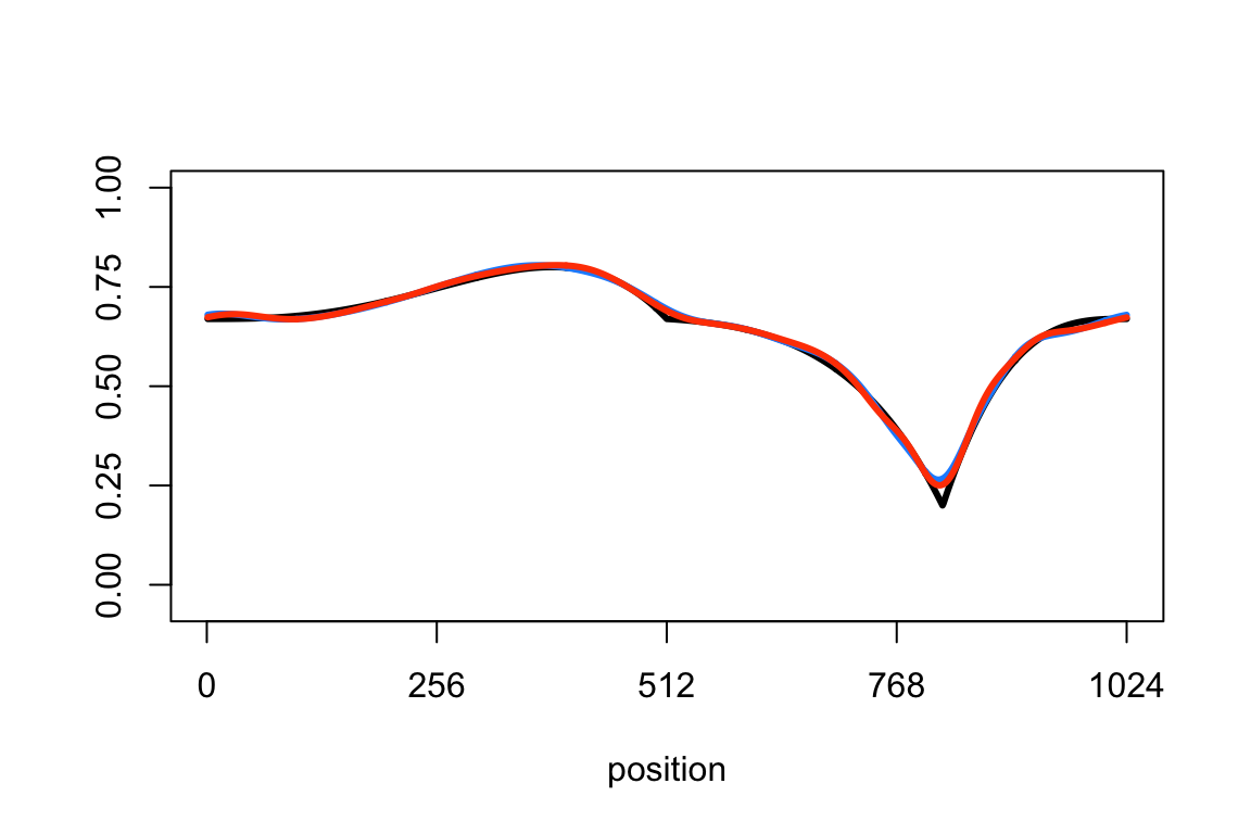
Extract the results from running these simulations.
hetero.data.smash.2 <-
  res[res$.id == "cor.3.v3" & res$method == "smash.s8",]
hetero.data.smash.homo.2 <-
  res[res$.id == "cor.3.v3" & res$method == "smash.homo.s8",]
hetero.data.tithresh.homo.2 <-
  res[res$.id == "cor.3.v3" & res$method == "tithresh.homo.s8",]
hetero.data.tithresh.rmad.2 <-
  res[res$.id == "cor.3.v3" & res$method == "tithresh.rmad.s8",]
hetero.data.tithresh.smash.2 <-
  res[res$.id == "cor.3.v3" & res$method == "tithresh.smash.s8",]
hetero.data.tithresh.true.2 <-
  res[res$.id == "cor.3.v3" & res$method == "tithresh.true.s8",]
hetero.data.ebayes.2 <-
  res[res$.id == "cor.3.v3" & res$method == "ebayesthresh",]
hetero.data.smash.true.2 <-
  res[res$.id == "cor.3.v3" & res$method == "smash.true.s8",]
Transform these results into a data frame suitable for ggplot2.
pdat <-
  rbind(data.frame(method      = "smash",
                   method.type = "est",
                   mise        = hetero.data.smash.2$mise),
        data.frame(method      = "smash.homo",
                   method.type = "homo",
                   mise        = hetero.data.smash.homo.2$mise),
        data.frame(method      = "tithresh.rmad",
                   method.type = "tithresh",
                   mise        = hetero.data.tithresh.rmad.2$mise),
        data.frame(method      = "tithresh.smash",
                   method.type = "tithresh",
                   mise        = hetero.data.tithresh.smash.2$mise),
        data.frame(method      = "tithresh.true",
                   method.type = "tithresh",
                   mise        = hetero.data.tithresh.true.2$mise),
        data.frame(method      = "ebayesthresh",
                   method.type = "homo",
                   mise        = hetero.data.ebayes.2$mise),
        data.frame(method      = "smash.true",
                   method.type = "true",
                   mise        = hetero.data.smash.true.2$mise))
pdat <-
  transform(pdat,
            method = factor(method,
                            names(sort(tapply(pdat$mise,pdat$method,mean),
                                       decreasing = TRUE))))
Create the combined boxplot and violin plot using ggplot2.
p <- ggplot(pdat,aes(x = method,y = mise,fill = method.type)) +
     geom_violin(fill = "skyblue",color = "skyblue") +
     geom_boxplot(width = 0.15,outlier.shape = NA) +
     scale_fill_manual(values=c("darkorange","dodgerblue","limegreen","gold"),
                       guide = FALSE) +
     coord_flip() +
     scale_y_continuous(breaks = seq(1,5)) +
     labs(x = "",y = "MISE") +
     theme(axis.line = element_blank(),
           axis.ticks.y = element_blank())
print(p)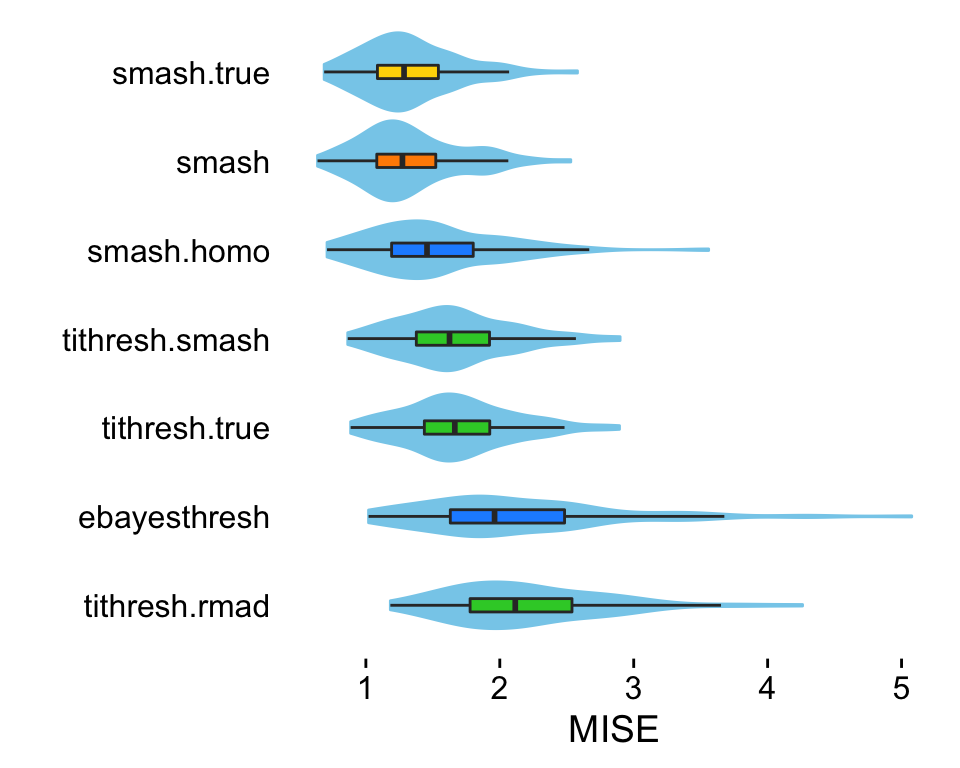
Similar to the “Spikes” scenario, we see that the SMASH method, when allowing for heteroskedastic variances, outperforms both the TI thresholding and EbayesThresh approaches.
Combined results from simulated data sets with heteroskedastic errors
These plots summarize the results from all combinations of test functions and a signal-to-noise ratio of 1.
create.bar.plots.heterosked(rbind(
  data.frame(mean="sp",  var="v2",get.results.heterosked(res,"sp.1.v2")),
  data.frame(mean="sp",  var="v3",get.results.heterosked(res,"sp.1.v3")),
  data.frame(mean="sp",  var="v4",get.results.heterosked(res,"sp.1.v4")),
  data.frame(mean="sp",  var="v5",get.results.heterosked(res,"sp.1.v5")),
  data.frame(mean="bump",var="v2",get.results.heterosked(res,"bump.1.v2")),
  data.frame(mean="bump",var="v3",get.results.heterosked(res,"bump.1.v3")),
  data.frame(mean="bump",var="v4",get.results.heterosked(res,"bump.1.v4")),
  data.frame(mean="bump",var="v5",get.results.heterosked(res,"bump.1.v5")),
  data.frame(mean="blk", var="v2",get.results.heterosked(res,"blk.1.v2")),
  data.frame(mean="blk", var="v3",get.results.heterosked(res,"blk.1.v3")),
  data.frame(mean="blk", var="v4",get.results.heterosked(res,"blk.1.v4")),
  data.frame(mean="blk", var="v5",get.results.heterosked(res,"blk.1.v5")),
  data.frame(mean="ang", var="v2",get.results.heterosked(res,"ang.1.v2")),
  data.frame(mean="ang", var="v3",get.results.heterosked(res,"ang.1.v3")),
  data.frame(mean="ang", var="v4",get.results.heterosked(res,"ang.1.v4")),
  data.frame(mean="ang", var="v5",get.results.heterosked(res,"ang.1.v5")),
  data.frame(mean="dop", var="v2",get.results.heterosked(res,"dop.1.v2")),
  data.frame(mean="dop", var="v3",get.results.heterosked(res,"dop.1.v3")),
  data.frame(mean="dop", var="v4",get.results.heterosked(res,"dop.1.v4")),
  data.frame(mean="dop", var="v5",get.results.heterosked(res,"dop.1.v5")),
  data.frame(mean="blip",var="v2",get.results.heterosked(res,"blip.1.v2")),
  data.frame(mean="blip",var="v3",get.results.heterosked(res,"blip.1.v3")),
  data.frame(mean="blip",var="v4",get.results.heterosked(res,"blip.1.v4")),
  data.frame(mean="blip",var="v5",get.results.heterosked(res,"blip.1.v5")),
  data.frame(mean="cor", var="v2",get.results.heterosked(res,"cor.1.v2")),
  data.frame(mean="cor", var="v3",get.results.heterosked(res,"cor.1.v3")),
  data.frame(mean="cor", var="v4",get.results.heterosked(res,"cor.1.v4")),
  data.frame(mean="cor", var="v5",get.results.heterosked(res,"cor.1.v5"))))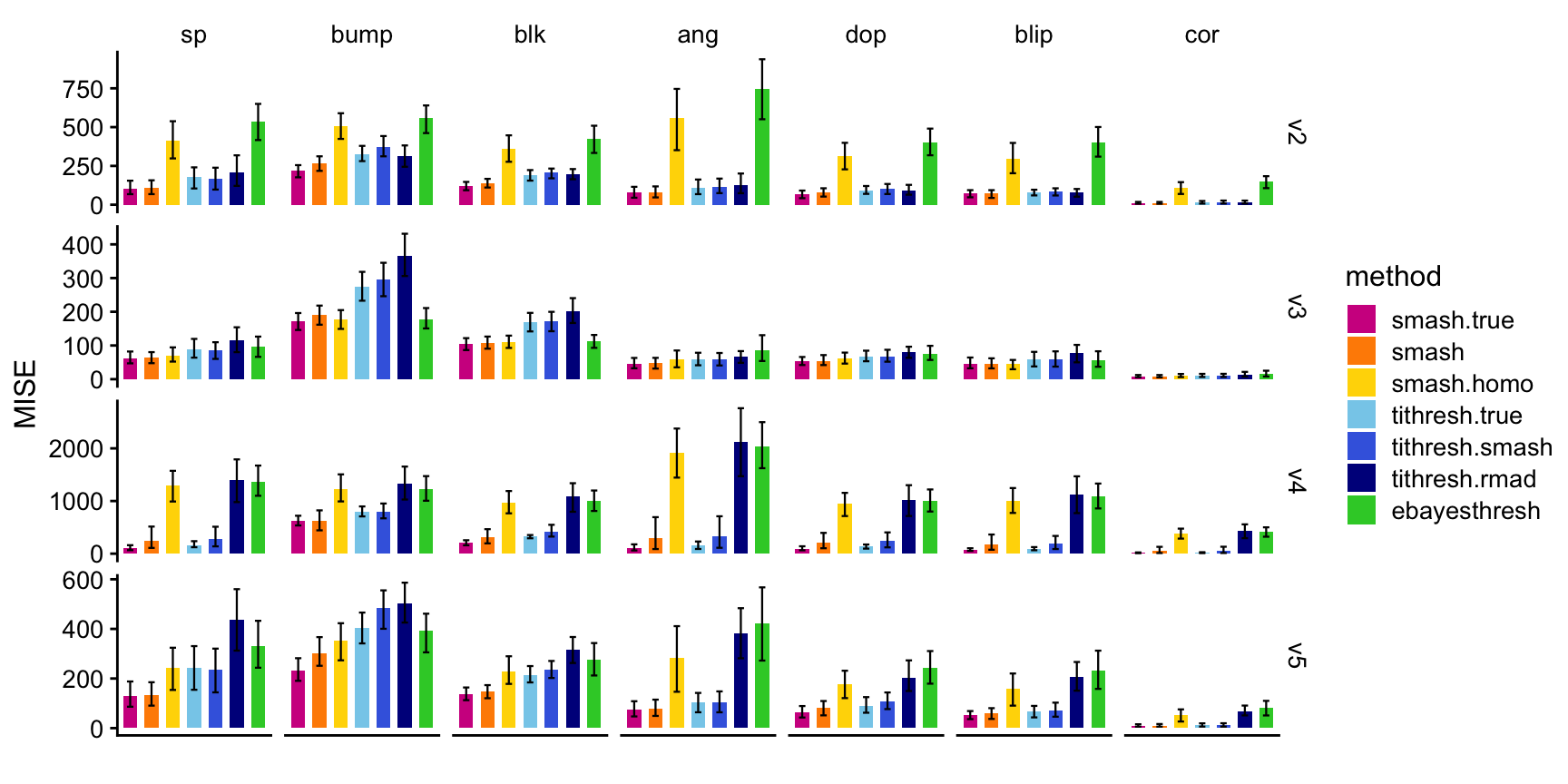
These plots summarize the results from data sets simulated using a signal-to-noise ratio of 3.
create.bar.plots.heterosked(rbind(
  data.frame(mean="sp",  var="v2",get.results.heterosked(res,"sp.3.v2")),
  data.frame(mean="sp",  var="v3",get.results.heterosked(res,"sp.3.v3")),
  data.frame(mean="sp",  var="v4",get.results.heterosked(res,"sp.3.v4")),
  data.frame(mean="sp",  var="v5",get.results.heterosked(res,"sp.3.v5")),
  data.frame(mean="bump",var="v2",get.results.heterosked(res,"bump.3.v2")),
  data.frame(mean="bump",var="v3",get.results.heterosked(res,"bump.3.v3")),
  data.frame(mean="bump",var="v4",get.results.heterosked(res,"bump.3.v4")),
  data.frame(mean="bump",var="v5",get.results.heterosked(res,"bump.3.v5")),
  data.frame(mean="blk", var="v2",get.results.heterosked(res,"blk.3.v2")),
  data.frame(mean="blk", var="v3",get.results.heterosked(res,"blk.3.v3")),
  data.frame(mean="blk", var="v4",get.results.heterosked(res,"blk.3.v4")),
  data.frame(mean="blk", var="v5",get.results.heterosked(res,"blk.3.v5")),
  data.frame(mean="ang", var="v2",get.results.heterosked(res,"ang.3.v2")),
  data.frame(mean="ang", var="v3",get.results.heterosked(res,"ang.3.v3")),
  data.frame(mean="ang", var="v4",get.results.heterosked(res,"ang.3.v4")),
  data.frame(mean="ang", var="v5",get.results.heterosked(res,"ang.3.v5")),
  data.frame(mean="dop", var="v2",get.results.heterosked(res,"dop.3.v2")),
  data.frame(mean="dop", var="v3",get.results.heterosked(res,"dop.3.v3")),
  data.frame(mean="dop", var="v4",get.results.heterosked(res,"dop.3.v4")),
  data.frame(mean="dop", var="v5",get.results.heterosked(res,"dop.3.v5")),
  data.frame(mean="blip",var="v2",get.results.heterosked(res,"blip.3.v2")),
  data.frame(mean="blip",var="v3",get.results.heterosked(res,"blip.3.v3")),
  data.frame(mean="blip",var="v4",get.results.heterosked(res,"blip.3.v4")),
  data.frame(mean="blip",var="v5",get.results.heterosked(res,"blip.3.v5")),
  data.frame(mean="cor", var="v2",get.results.heterosked(res,"cor.3.v2")),
  data.frame(mean="cor", var="v3",get.results.heterosked(res,"cor.3.v3")),
  data.frame(mean="cor", var="v4",get.results.heterosked(res,"cor.3.v4")),
  data.frame(mean="cor", var="v5",get.results.heterosked(res,"cor.3.v5"))))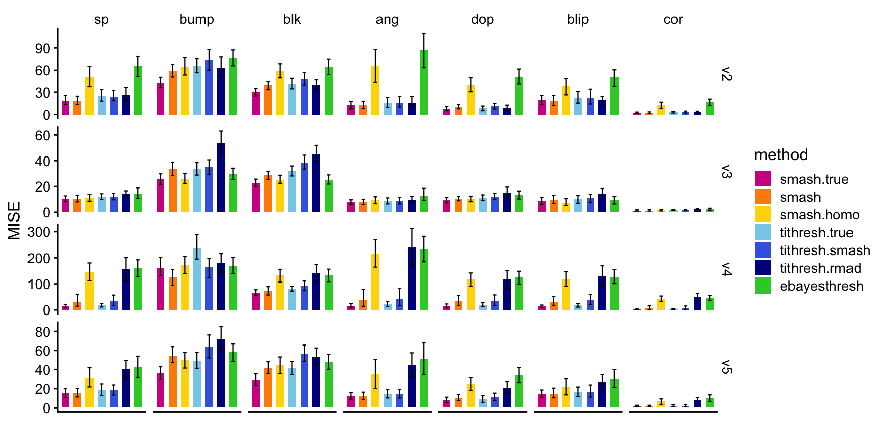
sessionInfo()
# R version 3.6.2 (2019-12-12)
# Platform: x86_64-apple-darwin15.6.0 (64-bit)
# Running under: macOS Catalina 10.15.5
#
# Matrix products: default
# BLAS:   /Library/Frameworks/R.framework/Versions/3.6/Resources/lib/libRblas.0.dylib
# LAPACK: /Library/Frameworks/R.framework/Versions/3.6/Resources/lib/libRlapack.dylib
#
# Random number generation:
#  RNG:     Mersenne-Twister
#  Normal:  Inversion
#  Sample:  Rounding
#
# locale:
# [1] en_US.UTF-8/en_US.UTF-8/en_US.UTF-8/C/en_US.UTF-8/en_US.UTF-8
#
# attached base packages:
# [1] stats     graphics  grDevices utils     datasets  methods   base
#
# other attached packages:
# [1] cowplot_1.0.0 ggplot2_3.3.0 smashr_1.2-5  plyr_1.8.5
#
# loaded via a namespace (and not attached):
#  [1] Rcpp_1.0.3        pillar_1.4.3      compiler_3.6.2    later_1.0.0
#  [5] git2r_0.26.1      workflowr_1.6.2   bitops_1.0-6      tools_3.6.2
#  [9] digest_0.6.23     tibble_2.1.3      lifecycle_0.1.0   evaluate_0.14
# [13] gtable_0.3.0      lattice_0.20-38   pkgconfig_2.0.3   rlang_0.4.5
# [17] Matrix_1.2-18     yaml_2.2.0        xfun_0.11         invgamma_1.1
# [21] withr_2.1.2       dplyr_0.8.3       stringr_1.4.0     knitr_1.26
# [25] fs_1.3.1          caTools_1.17.1.3  tidyselect_0.2.5  rprojroot_1.3-2
# [29] grid_3.6.2        glue_1.3.1        data.table_1.12.8 R6_2.4.1
# [33] rmarkdown_2.0     mixsqp_0.3-43     irlba_2.3.3       farver_2.0.1
# [37] purrr_0.3.3       ashr_2.2-50       magrittr_1.5      whisker_0.4
# [41] scales_1.1.0      backports_1.1.5   promises_1.1.0    htmltools_0.4.0
# [45] MASS_7.3-51.4     assertthat_0.2.1  colorspace_1.4-1  httpuv_1.5.2
# [49] labeling_0.3      wavethresh_4.6.8  stringi_1.4.3     munsell_0.5.0
# [53] truncnorm_1.0-8   SQUAREM_2017.10-1 crayon_1.3.4