ChIP-seq example

Last updated: 2019-12-18

Checks: 7 0

Knit directory: smash-paper/analysis/

This reproducible R Markdown analysis was created with workflowr (version 1.5.0.9000). The Checks tab describes the reproducibility checks that were applied when the results were created. The Past versions tab lists the development history.

R Markdown file: up-to-date

Great! Since the R Markdown file has been committed to the Git repository, you know the exact version of the code that produced these results.

Environment: empty

Great job! The global environment was empty. Objects defined in the global environment can affect the analysis in your R Markdown file in unknown ways. For reproduciblity it’s best to always run the code in an empty environment.

Seed: set.seed(1)

The command set.seed(1) was run prior to running the code in the R Markdown file. Setting a seed ensures that any results that rely on randomness, e.g. subsampling or permutations, are reproducible.

Session information: recorded

Great job! Recording the operating system, R version, and package versions is critical for reproducibility.

Cache: none

Nice! There were no cached chunks for this analysis, so you can be confident that you successfully produced the results during this run.

File paths: relative

Great job! Using relative paths to the files within your workflowr project makes it easier to run your code on other machines.

Repository version: 7f7b18d

Great! You are using Git for version control. Tracking code development and connecting the code version to the results is critical for reproducibility. The version displayed above was the version of the Git repository at the time these results were generated.

Note that you need to be careful to ensure that all relevant files for the analysis have been committed to Git prior to generating the results (you can use wflow_publish or wflow_git_commit). workflowr only checks the R Markdown file, but you know if there are other scripts or data files that it depends on. Below is the status of the Git repository when the results were generated:


Ignored files:
    Ignored:    dsc/code/Wavelab850/MEXSource/CPAnalysis.mexmac
    Ignored:    dsc/code/Wavelab850/MEXSource/DownDyadHi.mexmac
    Ignored:    dsc/code/Wavelab850/MEXSource/DownDyadLo.mexmac
    Ignored:    dsc/code/Wavelab850/MEXSource/FAIPT.mexmac
    Ignored:    dsc/code/Wavelab850/MEXSource/FCPSynthesis.mexmac
    Ignored:    dsc/code/Wavelab850/MEXSource/FMIPT.mexmac
    Ignored:    dsc/code/Wavelab850/MEXSource/FWPSynthesis.mexmac
    Ignored:    dsc/code/Wavelab850/MEXSource/FWT2_PO.mexmac
    Ignored:    dsc/code/Wavelab850/MEXSource/FWT_PBS.mexmac
    Ignored:    dsc/code/Wavelab850/MEXSource/FWT_PO.mexmac
    Ignored:    dsc/code/Wavelab850/MEXSource/FWT_TI.mexmac
    Ignored:    dsc/code/Wavelab850/MEXSource/IAIPT.mexmac
    Ignored:    dsc/code/Wavelab850/MEXSource/IMIPT.mexmac
    Ignored:    dsc/code/Wavelab850/MEXSource/IWT2_PO.mexmac
    Ignored:    dsc/code/Wavelab850/MEXSource/IWT_PBS.mexmac
    Ignored:    dsc/code/Wavelab850/MEXSource/IWT_PO.mexmac
    Ignored:    dsc/code/Wavelab850/MEXSource/IWT_TI.mexmac
    Ignored:    dsc/code/Wavelab850/MEXSource/LMIRefineSeq.mexmac
    Ignored:    dsc/code/Wavelab850/MEXSource/MedRefineSeq.mexmac
    Ignored:    dsc/code/Wavelab850/MEXSource/UpDyadHi.mexmac
    Ignored:    dsc/code/Wavelab850/MEXSource/UpDyadLo.mexmac
    Ignored:    dsc/code/Wavelab850/MEXSource/WPAnalysis.mexmac
    Ignored:    dsc/code/Wavelab850/MEXSource/dct_ii.mexmac
    Ignored:    dsc/code/Wavelab850/MEXSource/dct_iii.mexmac
    Ignored:    dsc/code/Wavelab850/MEXSource/dct_iv.mexmac
    Ignored:    dsc/code/Wavelab850/MEXSource/dst_ii.mexmac
    Ignored:    dsc/code/Wavelab850/MEXSource/dst_iii.mexmac

Untracked files:
    Untracked:  files.txt

Note that any generated files, e.g. HTML, png, CSS, etc., are not included in this status report because it is ok for generated content to have uncommitted changes.

These are the previous versions of the R Markdown and HTML files. If you’ve configured a remote Git repository (see ?wflow_git_remote), click on the hyperlinks in the table below to view them.

File	Version	Author	Date	Message
Rmd	7f7b18d	Peter Carbonetto	2019-12-18	Made a few small revisions to the text in the chipseq analysis.
html	2319196	Peter Carbonetto	2019-12-18	Re-built the chipseq analysis after adding the HF method and making
Rmd	e576395	Peter Carbonetto	2019-12-18	wflow_publish(“chipseq.Rmd”)
Rmd	f899adf	Peter Carbonetto	2019-12-18	Working on code to run HF method in chipseq example.
Rmd	500381a	Zhengrong Xing	2019-10-28	move gausdemo; add HF for chipseq
html	99d1f34	Peter Carbonetto	2018-12-07	Re-built all the outdated workflowr webpages.
Rmd	a09d13e	Peter Carbonetto	2018-11-09	Adjusted setup steps in a few of the R Markdown files.
html	0fa970b	Peter Carbonetto	2018-11-07	Some small adjustments to the chipseq example text.
Rmd	d9f6b81	Peter Carbonetto	2018-11-07	wflow_publish(“chipseq.Rmd”)
html	0b15924	Peter Carbonetto	2018-11-07	Added setup instructions to chipseq analysis.
Rmd	f5dec9c	Peter Carbonetto	2018-11-07	wflow_publish(“chipseq.Rmd”)
Rmd	f9f193c	Peter Carbonetto	2018-11-07	Revised setup instructions for a couple .Rmd files.
html	9cf40ea	Peter Carbonetto	2018-11-07	Build site.
Rmd	63bc42d	Peter Carbonetto	2018-11-07	wflow_publish(“chipseq.Rmd”)
html	b66089f	Peter Carbonetto	2018-10-19	Added a bit of explanatory text to the end of the chipseq.Rmd analysis.
Rmd	891e862	Peter Carbonetto	2018-10-19	wflow_publish(“chipseq.Rmd”)
html	f49c927	Peter Carbonetto	2018-10-18	Adjusted size of figure in chipseq example.
Rmd	3683070	Peter Carbonetto	2018-10-18	wflow_publish(“chipseq.Rmd”)
html	17b5a47	Peter Carbonetto	2018-10-18	Adjusted chipseq R Markdown source.
Rmd	38211a8	Peter Carbonetto	2018-10-18	wflow_publish(“chipseq.Rmd”)
html	b9c076d	Peter Carbonetto	2018-10-18	First wflow_publish(“chipseq.Rmd”).
Rmd	90e3ac9	Peter Carbonetto	2018-10-18	wflow_publish(“chipseq.Rmd”)
Rmd	1ef7492	Peter Carbonetto	2018-10-18	Working on chipseq R Markdown file.

This is an illustration of “SMoothing by Adaptive SHrinkage” (SMASH) applied to chromatin immunoprecipitation sequencing (“ChIP-seq”) data. This implements the SMASH analysis presented in Sec. 5.2 of the manuscript.

Initial setup instructions

To run this example on your own computer, please follow these setup instructions. These instructions assume you already have R (optionally, RStudio) installed on your computer.

Download or clone the git repository on your computer.

Launch R, and change the working directory to be the “analysis” folder inside your local copy of the git repository.

Install the devtools, ggplot2 and cowplot packages used here and in the code below:

install.packages(c("devtools","ggplot2","cowplot"))

Finally, install the smashr package from GitHub:

devtools::install_github("stephenslab/smashr")

See the “Session Info” at the bottom for the versions of the software and R packages that were used to generate the results shown below.

Set up R environment

Loading the smashr, ggplot2 and cowplot packages, as well as some additional functions used to implement the analysis below.

source("../code/chipseq.functions.R")
library(smashr)
library(ggplot2)
library(cowplot)
library(haarfisz)

Load the ChIP-seq data

The ChIP-seq data are sequencing read counts for transcription factor YY1 in cell line GM12878, restricted to 880,001–1,011,072 bp on chromosome 1. These data were collected as part of the ENCODE (“Encyclopedia Of DNA Elements”) project. The data are included with the git repository.

load("../data/reg_880000_1011072.RData")
bppos  <- 880001:1011072
counts <- M[1,] + M[,2]

Note that there are two replicates of the GM12878 cell line, so we analyze the combined read counts from both replicates, stored in the counts vectors.

Run SMASH and Haar-Fisz methods

The Haar-Fisz method transforms the Poisson counts, then applies Gaussian wavelet methods to the transformed data. Note that this call can take several minutes to run on a modern desktop computer.

res.hf <- denoise.poisson(counts,meth.1 = hf.la10.ti4,cs.1 = 50,hybrid = FALSE)

Next, we apply SMASH to the read counts to estimate the mean and variance of the underlying signal. It could also take several minutes to complete this step.

res <- smash.poiss(counts,post.var = TRUE)

Plot the SMASH and Haar-Fisz estimates

To provide a “baseline” to compare against the SMASH estimates, we retrieve the peaks identified in the same ChIP-seq data using the MACS software. Again, these data should have been included with the git repository you downloaded by following the instructions above.

macs.file <- "../data/Gm1287peaks_chr1_sorted.txt"
peaks <- read.macs.peaks(macs.file,min(bppos),max(bppos))

This next plot shows the intensity functions estimated by SMASH (orange line) and the Haar-Fisz method (dark blue line). The read count data are depicted as light blue circles, in which the area of each circle is scaled by the number of data points that fall within each 1.6-kb “bin”. (We show counts summarized within bins because there are too many data points to plot them individually.) The peaks identified by the MACS software are shown as red triangles. (Specifically, these are the mean positions of the identified peak intervals; the peak intervals are short enough that it is not useful to show both the start and end positions of these intervals.)

create.chipseq.plot(bppos/1e6,counts,res$est,res.hf,
                    (peaks$start + peaks$end)/2e6,nbreaks = 80) +
  scale_x_continuous(limits = c(0.88,1.02),breaks = seq(0.88,1.02,0.02)) +
  scale_y_continuous(limits = c(-1,9),breaks = seq(0,8,2))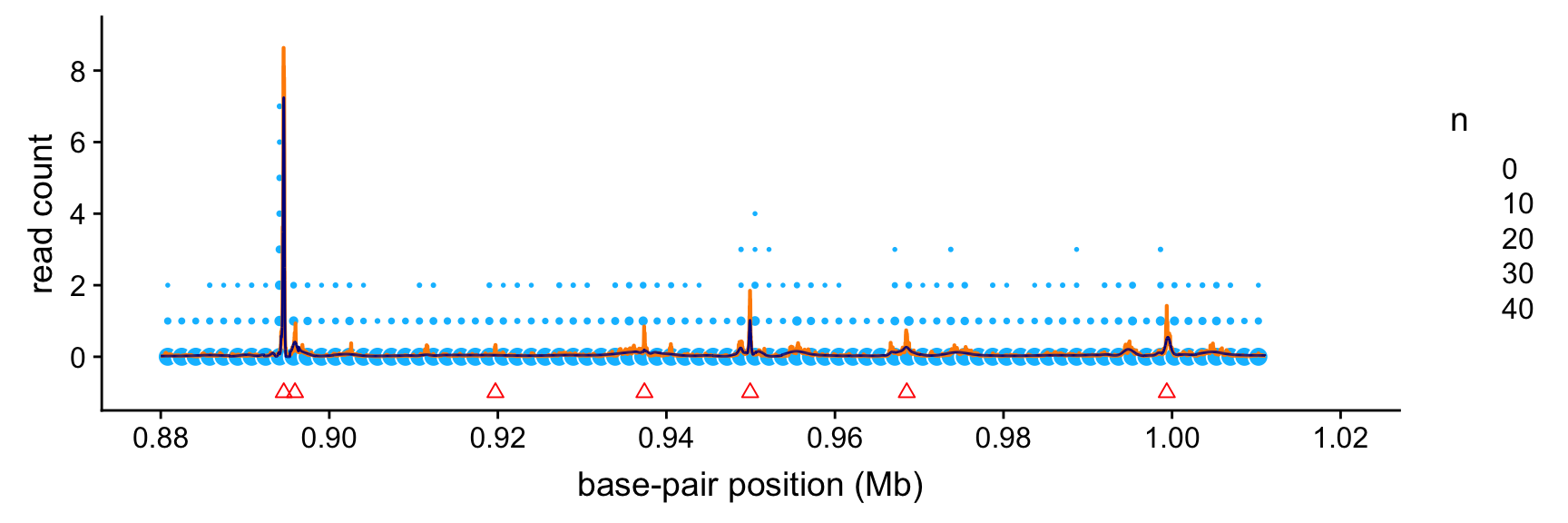

Version	Author	Date
2319196	Peter Carbonetto	2019-12-18
f49c927	Peter Carbonetto	2018-10-18
17b5a47	Peter Carbonetto	2018-10-18
b9c076d	Peter Carbonetto	2018-10-18

Based on this plot, it is clear that the strongest Haar-Fisz and SMASH intensity estimates align very closely with the peaks found by MACS, although the Haar-Fisz method failed to replicate at least two of the MACS peaks. Intriguingly, the SMASH estimates also suggest the presence of several additional weaker peaks that were not identified by MACS.